Python Data Science Handbook

(1)

Jake VanderPlas

Python

Data Science Handbook

ESSENTIAL TOOLS FOR WORKING WITH DATA

powered by

(2)

(3)

Jake VanderPlas

Python Data Science Handbook

Essential Tools for Working with Data

Boston Farnham Sebastopol Tokyo

Beijing Boston Farnham Sebastopol Tokyo

Beijing

(4)

978-1-491-91205-8 [LSI]

Python Data Science Handbook

by Jake VanderPlas

Printed in the United States of America.

Published by O’Reilly Media, Inc., 1005 Gravenstein Highway North, Sebastopol, CA 95472.

O’Reilly books may be purchased for educational, business, or sales promotional use. Online editions are also available for most titles (http://oreilly.com/safari). For more information, contact our corporate/insti‐

tutional sales department: 800-998-9938 or corporate@oreilly.com.

Editor: Dawn Schanafelt Production Editor: Kristen Brown Copyeditor: Jasmine Kwityn Proofreader: Rachel Monaghan

Indexer: WordCo Indexing Services, Inc.

Interior Designer: David Futato Cover Designer: Karen Montgomery Illustrator: Rebecca Demarest December 2016: First Edition

Revision History for the First Edition 2016-11-17: First Release

See http://oreilly.com/catalog/errata.csp?isbn=9781491912058 for release details.

The O’Reilly logo is a registered trademark of O’Reilly Media, Inc. Python Data Science Handbook, the cover image, and related trade dress are trademarks of O’Reilly Media, Inc.

While the publisher and the author have used good faith efforts to ensure that the information and instructions contained in this work are accurate, the publisher and the author disclaim all responsibility for errors or omissions, including without limitation responsibility for damages resulting from the use of or reliance on this work. Use of the information and instructions contained in this work is at your own risk. If any code samples or other technology this work contains or describes is subject to open source licenses or the intellectual property rights of others, it is your responsibility to ensure that your use thereof complies with such licenses and/or rights.

(5)

2. Introduction to NumPy. . . 33

Understanding Data Types in Python 34

A Python Integer Is More Than Just an Integer 35

A Python List Is More Than Just a List 37

Fixed-Type Arrays in Python 38

Creating Arrays from Python Lists 39

Creating Arrays from Scratch 39

NumPy Standard Data Types 41

The Basics of NumPy Arrays 42

NumPy Array Attributes 42

Array Indexing: Accessing Single Elements 43

Array Slicing: Accessing Subarrays 44

Reshaping of Arrays 47

Array Concatenation and Splitting 48

Computation on NumPy Arrays: Universal Functions 50

The Slowness of Loops 50

Introducing UFuncs 51

Exploring NumPy’s UFuncs 52

Advanced Ufunc Features 56

Ufuncs: Learning More 58

Aggregations: Min, Max, and Everything in Between 58

Summing the Values in an Array 59

Minimum and Maximum 59

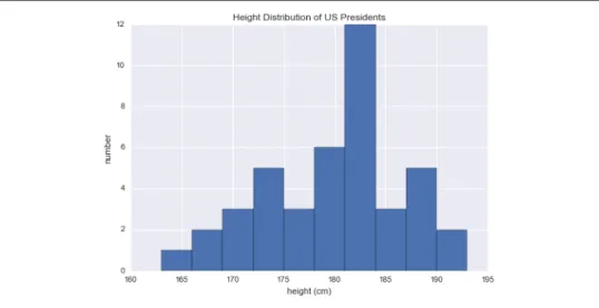
Example: What Is the Average Height of US Presidents? 61

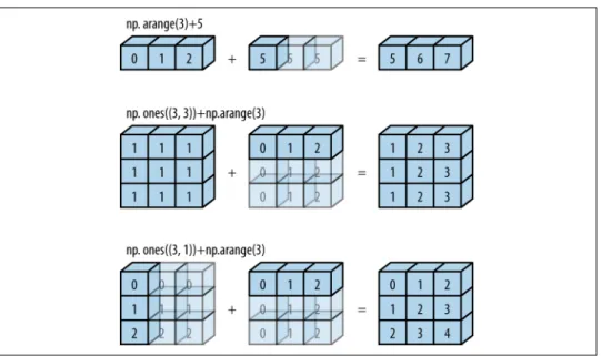
Computation on Arrays: Broadcasting 63

Introducing Broadcasting 63

Rules of Broadcasting 65

Broadcasting in Practice 68 iv | Table of Contents

(7)

Comparisons, Masks, and Boolean Logic 70

Example: Counting Rainy Days 70

Comparison Operators as ufuncs 71

Working with Boolean Arrays 73

Boolean Arrays as Masks 75

Fancy Indexing 78

Exploring Fancy Indexing 79

Combined Indexing 80

Example: Selecting Random Points 81

Modifying Values with Fancy Indexing 82

Example: Binning Data 83

Sorting Arrays 85

Fast Sorting in NumPy: np.sort and np.argsort 86

Partial Sorts: Partitioning 88

Example: k-Nearest Neighbors 88

Structured Data: NumPy’s Structured Arrays 92

Creating Structured Arrays 94

More Advanced Compound Types 95

RecordArrays: Structured Arrays with a Twist 96

On to Pandas 96

3. Data Manipulation with Pandas. . . 97

Installing and Using Pandas 97

Introducing Pandas Objects 98

The Pandas Series Object 99

The Pandas DataFrame Object 102

The Pandas Index Object 105

Data Indexing and Selection 107

Data Selection in Series 107

Data Selection in DataFrame 110

Operating on Data in Pandas 115

Ufuncs: Index Preservation 115

UFuncs: Index Alignment 116

Ufuncs: Operations Between DataFrame and Series 118

Handling Missing Data 119

Trade-Offs in Missing Data Conventions 120

Missing Data in Pandas 120

Operating on Null Values 124

Hierarchical Indexing 128

A Multiply Indexed Series 128

Methods of MultiIndex Creation 131

Indexing and Slicing a MultiIndex 134 Table of Contents | v

(8)

Rearranging Multi-Indices 137

Data Aggregations on Multi-Indices 140

Combining Datasets: Concat and Append 141

Recall: Concatenation of NumPy Arrays 142

Simple Concatenation with pd.concat 142

Combining Datasets: Merge and Join 146

Relational Algebra 146

Categories of Joins 147

Specification of the Merge Key 149

Specifying Set Arithmetic for Joins 152

Overlapping Column Names: The suffixes Keyword 153

Example: US States Data 154

Aggregation and Grouping 158

Planets Data 159

Simple Aggregation in Pandas 159

GroupBy: Split, Apply, Combine 161

Pivot Tables 170

Motivating Pivot Tables 170

Pivot Tables by Hand 171

Pivot Table Syntax 171

Example: Birthrate Data 174

Vectorized String Operations 178

Introducing Pandas String Operations 178

Tables of Pandas String Methods 180

Example: Recipe Database 184

Working with Time Series 188

Dates and Times in Python 188

Pandas Time Series: Indexing by Time 192

Pandas Time Series Data Structures 192

Frequencies and Offsets 195

Resampling, Shifting, and Windowing 196

Where to Learn More 202

Example: Visualizing Seattle Bicycle Counts 202

High-Performance Pandas: eval() and query() 208

Motivating query() and eval(): Compound Expressions 209

pandas.eval() for Efficient Operations 210

DataFrame.eval() for Column-Wise Operations 211

DataFrame.query() Method 213

Performance: When to Use These Functions 214

Further Resources 215

vi | Table of Contents

(9)

4. Visualization with Matplotlib. . . 217

General Matplotlib Tips 218

Importing matplotlib 218

Setting Styles 218

show() or No show()? How to Display Your Plots 218

Saving Figures to File 221

Two Interfaces for the Price of One 222

Simple Line Plots 224

Adjusting the Plot: Line Colors and Styles 226

Adjusting the Plot: Axes Limits 228

Labeling Plots 230

Simple Scatter Plots 233

Scatter Plots with plt.plot 233

Scatter Plots with plt.scatter 235

plot Versus scatter: A Note on Efficiency 237

Visualizing Errors 237

Basic Errorbars 238

Continuous Errors 239

Density and Contour Plots 241

Visualizing a Three-Dimensional Function 241

Histograms, Binnings, and Density 245

Two-Dimensional Histograms and Binnings 247

Customizing Plot Legends 249

Choosing Elements for the Legend 251

Legend for Size of Points 252

Multiple Legends 254

Customizing Colorbars 255

Customizing Colorbars 256

Example: Handwritten Digits 261

Multiple Subplots 262

plt.axes: Subplots by Hand 263

plt.subplot: Simple Grids of Subplots 264

plt.subplots: The Whole Grid in One Go 265

plt.GridSpec: More Complicated Arrangements 266

Text and Annotation 268

Example: Effect of Holidays on US Births 269

Transforms and Text Position 270

Arrows and Annotation 272

Customizing Ticks 275

Major and Minor Ticks 276

Hiding Ticks or Labels 277

Reducing or Increasing the Number of Ticks 278 Table of Contents | vii

(10)

Fancy Tick Formats 279

Summary of Formatters and Locators 281

Customizing Matplotlib: Configurations and Stylesheets 282

Plot Customization by Hand 282

Changing the Defaults: rcParams 284

Stylesheets 285

Three-Dimensional Plotting in Matplotlib 290

Three-Dimensional Points and Lines 291

Three-Dimensional Contour Plots 292

Wireframes and Surface Plots 293

Surface Triangulations 295

Geographic Data with Basemap 298

Map Projections 300

Drawing a Map Background 304

Plotting Data on Maps 307

Example: California Cities 308

Example: Surface Temperature Data 309

Visualization with Seaborn 311

Seaborn Versus Matplotlib 312

Exploring Seaborn Plots 313

Example: Exploring Marathon Finishing Times 322

Further Resources 329

Matplotlib Resources 329

Other Python Graphics Libraries 330

5. Machine Learning. . . 331

What Is Machine Learning? 332

Categories of Machine Learning 332

Qualitative Examples of Machine Learning Applications 333

Summary 342

Introducing Scikit-Learn 343

Data Representation in Scikit-Learn 343

Scikit-Learn’s Estimator API 346

Application: Exploring Handwritten Digits 354

Summary 359

Hyperparameters and Model Validation 359

Thinking About Model Validation 359

Selecting the Best Model 363

Learning Curves 370

Validation in Practice: Grid Search 373

Summary 375

Feature Engineering 375 viii | Table of Contents

(11)

Categorical Features 376

Text Features 377

Image Features 378

Derived Features 378

Imputation of Missing Data 381

Feature Pipelines 381

In Depth: Naive Bayes Classification 382

Bayesian Classification 383

Gaussian Naive Bayes 383

Multinomial Naive Bayes 386

When to Use Naive Bayes 389

In Depth: Linear Regression 390

Simple Linear Regression 390

Basis Function Regression 392

Regularization 396

Example: Predicting Bicycle Traffic 400

In-Depth: Support Vector Machines 405

Motivating Support Vector Machines 405

Support Vector Machines: Maximizing the Margin 407

Example: Face Recognition 416

Support Vector Machine Summary 420

In-Depth: Decision Trees and Random Forests 421

Motivating Random Forests: Decision Trees 421

Ensembles of Estimators: Random Forests 426

Random Forest Regression 428

Example: Random Forest for Classifying Digits 430

Summary of Random Forests 432

In Depth: Principal Component Analysis 433

Introducing Principal Component Analysis 433

PCA as Noise Filtering 440

Example: Eigenfaces 442

Principal Component Analysis Summary 445

In-Depth: Manifold Learning 445

Manifold Learning: “HELLO” 446

Multidimensional Scaling (MDS) 447

MDS as Manifold Learning 450

Nonlinear Embeddings: Where MDS Fails 452

Nonlinear Manifolds: Locally Linear Embedding 453

Some Thoughts on Manifold Methods 455

Example: Isomap on Faces 456

Example: Visualizing Structure in Digits 460

In Depth: k-Means Clustering 462 Table of Contents | ix

(12)

Introducing k-Means 463

k-Means Algorithm: Expectation–Maximization 465

Examples 470

In Depth: Gaussian Mixture Models 476

Motivating GMM: Weaknesses of k-Means 477

Generalizing E–M: Gaussian Mixture Models 480

GMM as Density Estimation 484

Example: GMM for Generating New Data 488

In-Depth: Kernel Density Estimation 491

Motivating KDE: Histograms 491

Kernel Density Estimation in Practice 496

Example: KDE on a Sphere 498

Example: Not-So-Naive Bayes 501

Application: A Face Detection Pipeline 506

HOG Features 506

HOG in Action: A Simple Face Detector 507

Caveats and Improvements 512

Further Machine Learning Resources 514

Machine Learning in Python 514

General Machine Learning 515

Index. . . 517

x | Table of Contents

(13)

Preface

What Is Data Science?

This is a book about doing data science with Python, which immediately begs the question: what is data science? It’s a surprisingly hard definition to nail down, espe‐

cially given how ubiquitous the term has become. Vocal critics have variously dis‐

missed the term as a superfluous label (after all, what science doesn’t involve data?) or a simple buzzword that only exists to salt résumés and catch the eye of overzealous tech recruiters.

In my mind, these critiques miss something important. Data science, despite its hype- laden veneer, is perhaps the best label we have for the cross-disciplinary set of skills that are becoming increasingly important in many applications across industry and academia. This cross-disciplinary piece is key: in my mind, the best existing defini‐

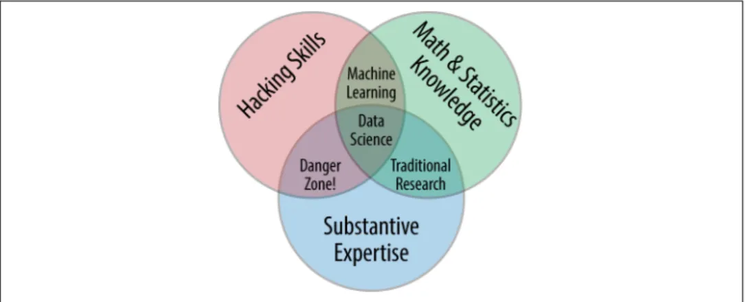
tion of data science is illustrated by Drew Conway’s Data Science Venn Diagram, first published on his blog in September 2010 (see Figure P-1).

Figure P-1. Drew Conway’s Data Science Venn Diagram

xi

(14)

While some of the intersection labels are a bit tongue-in-cheek, this diagram captures the essence of what I think people mean when they say “data science”: it is fundamen‐

tally an interdisciplinary subject. Data science comprises three distinct and overlap‐

ping areas: the skills of a statistician who knows how to model and summarize datasets (which are growing ever larger); the skills of a computer scientist who can design and use algorithms to efficiently store, process, and visualize this data; and the domain expertise—what we might think of as “classical” training in a subject—neces‐

sary both to formulate the right questions and to put their answers in context.

With this in mind, I would encourage you to think of data science not as a new domain of knowledge to learn, but as a new set of skills that you can apply within your current area of expertise. Whether you are reporting election results, forecasting stock returns, optimizing online ad clicks, identifying microorganisms in microscope photos, seeking new classes of astronomical objects, or working with data in any other field, the goal of this book is to give you the ability to ask and answer new ques‐

tions about your chosen subject area.

Who Is This Book For?

In my teaching both at the University of Washington and at various tech-focused conferences and meetups, one of the most common questions I have heard is this:

“how should I learn Python?” The people asking are generally technically minded students, developers, or researchers, often with an already strong background in writ‐

ing code and using computational and numerical tools. Most of these folks don’t want to learn Python per se, but want to learn the language with the aim of using it as a tool for data-intensive and computational science. While a large patchwork of videos, blog posts, and tutorials for this audience is available online, I’ve long been frustrated by the lack of a single good answer to this question; that is what inspired this book.

The book is not meant to be an introduction to Python or to programming in gen‐

eral; I assume the reader has familiarity with the Python language, including defining functions, assigning variables, calling methods of objects, controlling the flow of a program, and other basic tasks. Instead, it is meant to help Python users learn to use Python’s data science stack—libraries such as IPython, NumPy, Pandas, Matplotlib, Scikit-Learn, and related tools—to effectively store, manipulate, and gain insight from data.

Why Python?

Python has emerged over the last couple decades as a first-class tool for scientific computing tasks, including the analysis and visualization of large datasets. This may have come as a surprise to early proponents of the Python language: the language itself was not specifically designed with data analysis or scientific computing in mind.

xii | Preface

(15)

The usefulness of Python for data science stems primarily from the large and active ecosystem of third-party packages: NumPy for manipulation of homogeneous array- based data, Pandas for manipulation of heterogeneous and labeled data, SciPy for common scientific computing tasks, Matplotlib for publication-quality visualizations, IPython for interactive execution and sharing of code, Scikit-Learn for machine learning, and many more tools that will be mentioned in the following pages.

If you are looking for a guide to the Python language itself, I would suggest the sister project to this book, A Whirlwind Tour of the Python Language. This short report pro‐

vides a tour of the essential features of the Python language, aimed at data scientists who already are familiar with one or more other programming languages.

Python 2 Versus Python 3

This book uses the syntax of Python 3, which contains language enhancements that are not compatible with the 2.x series of Python. Though Python 3.0 was first released in 2008, adoption has been relatively slow, particularly in the scientific and web devel‐

opment communities. This is primarily because it took some time for many of the essential third-party packages and toolkits to be made compatible with the new lan‐

guage internals. Since early 2014, however, stable releases of the most important tools in the data science ecosystem have been fully compatible with both Python 2 and 3, and so this book will use the newer Python 3 syntax. However, the vast majority of code snippets in this book will also work without modification in Python 2: in cases where a Py2-incompatible syntax is used, I will make every effort to note it explicitly.

Outline of This Book

Each chapter of this book focuses on a particular package or tool that contributes a fundamental piece of the Python data science story.

IPython and Jupyter (Chapter 1)

These packages provide the computational environment in which many Python- using data scientists work.

NumPy (Chapter 2)

This library provides the ^ndarray object for efficient storage and manipulation of dense data arrays in Python.

Pandas (Chapter 3)

This library provides the ^DataFrame object for efficient storage and manipulation of labeled/columnar data in Python.

Matplotlib (Chapter 4)

This library provides capabilities for a flexible range of data visualizations in Python.

Preface | xiii

(16)

Scikit-Learn (Chapter 5)

This library provides efficient and clean Python implementations of the most important and established machine learning algorithms.

The PyData world is certainly much larger than these five packages, and is growing every day. With this in mind, I make every attempt through these pages to provide references to other interesting efforts, projects, and packages that are pushing the boundaries of what can be done in Python. Nevertheless, these five are currently fun‐

damental to much of the work being done in the Python data science space, and I expect they will remain important even as the ecosystem continues growing around them.

Using Code Examples

Supplemental material (code examples, figures, etc.) is available for download at https://github.com/jakevdp/PythonDataScienceHandbook. This book is here to help you get your job done. In general, if example code is offered with this book, you may use it in your programs and documentation. You do not need to contact us for per‐

mission unless you’re reproducing a significant portion of the code. For example, writing a program that uses several chunks of code from this book does not require permission. Selling or distributing a CD-ROM of examples from O’Reilly books does require permission. Answering a question by citing this book and quoting example code does not require permission. Incorporating a significant amount of example code from this book into your product’s documentation does require permission.

We appreciate, but do not require, attribution. An attribution usually includes the title, author, publisher, and ISBN. For example, “Python Data Science Handbook by Jake VanderPlas (O’Reilly). Copyright 2017 Jake VanderPlas, 978-1-491-91205-8.”

If you feel your use of code examples falls outside fair use or the permission given above, feel free to contact us at permissions@oreilly.com.

Installation Considerations

Installing Python and the suite of libraries that enable scientific computing is straightforward. This section will outline some of the considerations to keep in mind when setting up your computer.

Though there are various ways to install Python, the one I would suggest for use in data science is the Anaconda distribution, which works similarly whether you use Windows, Linux, or Mac OS X. The Anaconda distribution comes in two flavors:

• Miniconda gives you the Python interpreter itself, along with a command-line tool called conda that operates as a cross-platform package manager geared

xiv | Preface

(17)

toward Python packages, similar in spirit to the apt or yum tools that Linux users might be familiar with.

• Anaconda includes both Python and conda, and additionally bundles a suite of other preinstalled packages geared toward scientific computing. Because of the size of this bundle, expect the installation to consume several gigabytes of disk space.

Any of the packages included with Anaconda can also be installed manually on top of Miniconda; for this reason I suggest starting with Miniconda.

To get started, download and install the Miniconda package (make sure to choose a version with Python 3), and then install the core packages used in this book:

[~]$ conda install numpy pandas scikit-learn matplotlib seaborn ipython-notebook

Throughout the text, we will also make use of other, more specialized tools in Python’s scientific ecosystem; installation is usually as easy as typing conda install packagename. For more information on conda, including information about creating and using conda environments (which I would highly recommend), refer to conda’s online documentation.

Conventions Used in This Book

The following typographical conventions are used in this book:

Italic

Indicates new terms, URLs, email addresses, filenames, and file extensions.

Constant width

Used for program listings, as well as within paragraphs to refer to program ele‐

ments such as variable or function names, databases, data types, environment variables, statements, and keywords.

Constant width bold

Shows commands or other text that should be typed literally by the user.

Constant width italic

Shows text that should be replaced with user-supplied values or by values deter‐

mined by context.

O’Reilly Safari

Safari (formerly Safari Books Online) is a membership-based training and reference platform for enterprise, government, educators, and individuals.

Preface | xv

(18)

Members have access to thousands of books, training videos, Learning Paths, interac‐

tive tutorials, and curated playlists from over 250 publishers, including O’Reilly Media, Harvard Business Review, Prentice Hall Professional, Addison-Wesley Profes‐

sional, Microsoft Press, Sams, Que, Peachpit Press, Adobe, Focal Press, Cisco Press, John Wiley & Sons, Syngress, Morgan Kaufmann, IBM Redbooks, Packt, Adobe Press, FT Press, Apress, Manning, New Riders, McGraw-Hill, Jones & Bartlett, and Course Technology, among others.

For more information, please visit http://oreilly.com/safari.

How to Contact Us

Please address comments and questions concerning this book to the publisher:

O’Reilly Media, Inc.

1005 Gravenstein Highway North Sebastopol, CA 95472

800-998-9938 (in the United States or Canada) 707-829-0515 (international or local)

707-829-0104 (fax)

We have a web page for this book, where we list errata, examples, and any additional information. You can access this page at http://bit.ly/python-data-sci-handbook.

To comment or ask technical questions about this book, send email to bookques‐

tions@oreilly.com.

For more information about our books, courses, conferences, and news, see our web‐

site at http://www.oreilly.com.

Find us on Facebook: http://facebook.com/oreilly Follow us on Twitter: http://twitter.com/oreillymedia Watch us on YouTube: http://www.youtube.com/oreillymedia

xvi | Preface

(19)

CHAPTER 1

IPython: Beyond Normal Python

There are many options for development environments for Python, and I’m often asked which one I use in my own work. My answer sometimes surprises people: my preferred environment is IPython plus a text editor (in my case, Emacs or Atom depending on my mood). IPython (short for Interactive Python) was started in 2001 by Fernando Perez as an enhanced Python interpreter, and has since grown into a project aiming to provide, in Perez’s words, “Tools for the entire lifecycle of research computing.” If Python is the engine of our data science task, you might think of IPy‐

thon as the interactive control panel.

As well as being a useful interactive interface to Python, IPython also provides a number of useful syntactic additions to the language; we’ll cover the most useful of these additions here. In addition, IPython is closely tied with the Jupyter project, which provides a browser-based notebook that is useful for development, collabora‐

tion, sharing, and even publication of data science results. The IPython notebook is actually a special case of the broader Jupyter notebook structure, which encompasses notebooks for Julia, R, and other programming languages. As an example of the use‐

fulness of the notebook format, look no further than the page you are reading: the entire manuscript for this book was composed as a set of IPython notebooks.

IPython is about using Python effectively for interactive scientific and data-intensive computing. This chapter will start by stepping through some of the IPython features that are useful to the practice of data science, focusing especially on the syntax it offers beyond the standard features of Python. Next, we will go into a bit more depth on some of the more useful “magic commands” that can speed up common tasks in creating and using data science code. Finally, we will touch on some of the features of the notebook that make it useful in understanding data and sharing results.

1

(20)

Shell or Notebook?

There are two primary means of using IPython that we’ll discuss in this chapter: the IPython shell and the IPython notebook. The bulk of the material in this chapter is relevant to both, and the examples will switch between them depending on what is most convenient. In the few sections that are relevant to just one or the other, I will explicitly state that fact. Before we start, some words on how to launch the IPython shell and IPython notebook.

Launching the IPython Shell

This chapter, like most of this book, is not designed to be absorbed passively. I recom‐

mend that as you read through it, you follow along and experiment with the tools and syntax we cover: the muscle-memory you build through doing this will be far more useful than the simple act of reading about it. Start by launching the IPython inter‐

preter by typing ^ipython on the command line; alternatively, if you’ve installed a dis‐

tribution like Anaconda or EPD, there may be a launcher specific to your system (we’ll discuss this more fully in “Help and Documentation in IPython” on page 3).

Once you do this, you should see a prompt like the following:

IPython 4.0.1 -- An enhanced Interactive Python.

? -> Introduction and overview of IPython's features.

%quickref -> Quick reference.

help -> Python's own help system.

object? -> Details about 'object', use 'object??' for extra details.

In [1]:

With that, you’re ready to follow along.

Launching the Jupyter Notebook

The Jupyter notebook is a browser-based graphical interface to the IPython shell, and builds on it a rich set of dynamic display capabilities. As well as executing Python/

IPython statements, the notebook allows the user to include formatted text, static and dynamic visualizations, mathematical equations, JavaScript widgets, and much more.

Furthermore, these documents can be saved in a way that lets other people open them and execute the code on their own systems.

Though the IPython notebook is viewed and edited through your web browser win‐

dow, it must connect to a running Python process in order to execute code. To start this process (known as a “kernel”), run the following command in your system shell:

$ jupyter notebook

This command will launch a local web server that will be visible to your browser. It immediately spits out a log showing what it is doing; that log will look something like this:

2 | Chapter 1: IPython: Beyond Normal Python

(21)

$ jupyter notebook

[NotebookApp] Serving notebooks from local directory: /Users/jakevdp/...

[NotebookApp] 0 active kernels

[NotebookApp] The IPython Notebook is running at: http://localhost:8888/

[NotebookApp] Use Control-C to stop this server and shut down all kernels...

Upon issuing the command, your default browser should automatically open and navigate to the listed local URL; the exact address will depend on your system. If the browser does not open automatically, you can open a window and manually open this address (http://localhost:8888/ in this example).

Help and Documentation in IPython

If you read no other section in this chapter, read this one: I find the tools discussed here to be the most transformative contributions of IPython to my daily workflow.

When a technologically minded person is asked to help a friend, family member, or colleague with a computer problem, most of the time it’s less a matter of knowing the answer as much as knowing how to quickly find an unknown answer. In data science it’s the same: searchable web resources such as online documentation, mailing-list threads, and Stack Overflow answers contain a wealth of information, even (espe‐

cially?) if it is a topic you’ve found yourself searching before. Being an effective prac‐

titioner of data science is less about memorizing the tool or command you should use for every possible situation, and more about learning to effectively find the informa‐

tion you don’t know, whether through a web search engine or another means.

One of the most useful functions of IPython/Jupyter is to shorten the gap between the user and the type of documentation and search that will help them do their work effectively. While web searches still play a role in answering complicated questions, an amazing amount of information can be found through IPython alone. Some examples of the questions IPython can help answer in a few keystrokes:

• How do I call this function? What arguments and options does it have?

• What does the source code of this Python object look like?

• What is in this package I imported? What attributes or methods does this object have?

Here we’ll discuss IPython’s tools to quickly access this information, namely the ^? character to explore documentation, the ^?? characters to explore source code, and the Tab key for autocompletion.

Accessing Documentation with ?

The Python language and its data science ecosystem are built with the user in mind, and one big part of that is access to documentation. Every Python object contains the

Help and Documentation in IPython | 3

(22)

reference to a string, known as a docstring, which in most cases will contain a concise summary of the object and how to use it. Python has a built-in ^help() function that can access this information and print the results. For example, to see the documenta‐

tion of the built-in ^len function, you can do the following:

In [1]: help(len)

Help on built-in function len in module builtins:

len(...)

len(object) -> integer

Return the number of items of a sequence or mapping.

Depending on your interpreter, this information may be displayed as inline text, or in some separate pop-up window.

Because finding help on an object is so common and useful, IPython introduces the ^? character as a shorthand for accessing this documentation and other relevant information:

In [2]: len?

Type: builtin_function_or_method String form: <built-in function len>

Namespace: Python builtin Docstring:

This notation works for just about anything, including object methods:

In [3]: L = [1, 2, 3]

In [4]: L.insert?

Type: builtin_function_or_method

String form: <built-in method insert of list object at 0x1024b8ea8>

Docstring: L.insert(index, object) -- insert object before index

or even objects themselves, with the documentation from their type:

In [5]: L?

Type: list String form: [1, 2, 3]

Length: 3 Docstring:

list() -> new empty list

list(iterable) -> new list initialized from iterable's items

Importantly, this will even work for functions or other objects you create yourself!

Here we’ll define a small function with a docstring:

In [6]: def square(a):

....: """Return the square of a."""

(23)

....: return a ** 2 ....:

Note that to create a docstring for our function, we simply placed a string literal in the first line. Because docstrings are usually multiple lines, by convention we used Python’s triple-quote notation for multiline strings.

Now we’ll use the ^? mark to find this docstring:

In [7]: square?

Type: function

String form: <function square at 0x103713cb0>

Definition: square(a)

Docstring: Return the square of a.

This quick access to documentation via docstrings is one reason you should get in the habit of always adding such inline documentation to the code you write!

Accessing Source Code with ??

Because the Python language is so easily readable, you can usually gain another level of insight by reading the source code of the object you’re curious about. IPython pro‐

vides a shortcut to the source code with the double question mark (^??):

In [8]: square??

Type: function

String form: <function square at 0x103713cb0>

Definition: square(a) Source:

def square(a):

"Return the square of a"

return a ** 2

For simple functions like this, the double question mark can give quick insight into the under-the-hood details.

If you play with this much, you’ll notice that sometimes the ^?? suffix doesn’t display any source code: this is generally because the object in question is not implemented in Python, but in C or some other compiled extension language. If this is the case, the ^??

suffix gives the same output as the ^? suffix. You’ll find this particularly with many of Python’s built-in objects and types, for example ^len from above:

In [9]: len??

Type: builtin_function_or_method String form: <built-in function len>

Namespace: Python builtin Docstring:

(24)

Using ^? and/or ^?? gives a powerful and quick interface for finding information about what any Python function or module does.

Exploring Modules with Tab Completion

IPython’s other useful interface is the use of the Tab key for autocompletion and exploration of the contents of objects, modules, and namespaces. In the examples that follow, we’ll use <TAB> to indicate when the Tab key should be pressed.

Tab completion of object contents

Every Python object has various attributes and methods associated with it. Like with the ^help function discussed before, Python has a built-in ^dir function that returns a list of these, but the tab-completion interface is much easier to use in practice. To see a list of all available attributes of an object, you can type the name of the object fol‐

lowed by a period (^.) character and the Tab key:

In [10]: L.<TAB>

L.append L.copy L.extend L.insert L.remove L.sort L.clear L.count L.index L.pop L.reverse

To narrow down the list, you can type the first character or several characters of the name, and the Tab key will find the matching attributes and methods:

In [10]: L.c<TAB>

L.clear L.copy L.count In [10]: L.co<TAB>

L.copy L.count

If there is only a single option, pressing the Tab key will complete the line for you. For example, the following will instantly be replaced with ^L.count:

In [10]: L.cou<TAB>

Though Python has no strictly enforced distinction between public/external attributes and private/internal attributes, by convention a preceding underscore is used to denote such methods. For clarity, these private methods and special methods are omitted from the list by default, but it’s possible to list them by explicitly typing the underscore:

In [10]: L._<TAB>

L.__add__ L.__gt__ L.__reduce__

L.__class__ L.__hash__ L.__reduce_ex__

For brevity, we’ve only shown the first couple lines of the output. Most of these are Python’s special double-underscore methods (often nicknamed “dunder” methods).

(25)

Tab completion when importing

Tab completion is also useful when importing objects from packages. Here we’ll use it to find all possible imports in the ^itertools package that start with ^co:

In [10]: from itertools import co<TAB>

combinations compress combinations_with_replacement count

Similarly, you can use tab completion to see which imports are available on your sys‐

tem (this will change depending on which third-party scripts and modules are visible to your Python session):

In [10]: import <TAB>

Display all 399 possibilities? (y or n)

Crypto dis py_compile Cython distutils pyclbr ... ... ...

difflib pwd zmq In [10]: import h<TAB>

hashlib hmac http heapq html husl

(Note that for brevity, I did not print here all 399 importable packages and modules on my system.)

Beyond tab completion: Wildcard matching

Tab completion is useful if you know the first few characters of the object or attribute you’re looking for, but is little help if you’d like to match characters at the middle or end of the word. For this use case, IPython provides a means of wildcard matching for names using the ^* character.

For example, we can use this to list every object in the namespace that ends with Warning:

In [10]: *Warning?

BytesWarning RuntimeWarning DeprecationWarning SyntaxWarning FutureWarning UnicodeWarning ImportWarning UserWarning PendingDeprecationWarning Warning ResourceWarning

Notice that the ^* character matches any string, including the empty string.

Similarly, suppose we are looking for a string method that contains the word ^find somewhere in its name. We can search for it this way:

(26)

In [10]: str.*find*?

str.find str.rfind

I find this type of flexible wildcard search can be very useful for finding a particular command when I’m getting to know a new package or reacquainting myself with a familiar one.

Keyboard Shortcuts in the IPython Shell

If you spend any amount of time on the computer, you’ve probably found a use for keyboard shortcuts in your workflow. Most familiar perhaps are Cmd-C and Cmd-V (or Ctrl-C and Ctrl-V) for copying and pasting in a wide variety of programs and sys‐

tems. Power users tend to go even further: popular text editors like Emacs, Vim, and others provide users an incredible range of operations through intricate combina‐

tions of keystrokes.

The IPython shell doesn’t go this far, but does provide a number of keyboard short‐

cuts for fast navigation while you’re typing commands. These shortcuts are not in fact provided by IPython itself, but through its dependency on the GNU Readline library:

thus, some of the following shortcuts may differ depending on your system configu‐

ration. Also, while some of these shortcuts do work in the browser-based notebook, this section is primarily about shortcuts in the IPython shell.

Once you get accustomed to these, they can be very useful for quickly performing certain commands without moving your hands from the “home” keyboard position.

If you’re an Emacs user or if you have experience with Linux-style shells, the follow‐

ing will be very familiar. We’ll group these shortcuts into a few categories: navigation shortcuts, text entry shortcuts, command history shortcuts, and miscellaneous shortcuts.

Navigation Shortcuts

While the use of the left and right arrow keys to move backward and forward in the line is quite obvious, there are other options that don’t require moving your hands from the “home” keyboard position:

Keystroke Action

Ctrl-a Move cursor to the beginning of the line

Ctrl-e Move cursor to the end of the line

Ctrl-b (or the left arrow key) Move cursor back one character Ctrl-f (or the right arrow key) Move cursor forward one character

(27)

Text Entry Shortcuts

While everyone is familiar with using the Backspace key to delete the previous char‐

acter, reaching for the key often requires some minor finger gymnastics, and it only deletes a single character at a time. In IPython there are several shortcuts for remov‐

ing some portion of the text you’re typing. The most immediately useful of these are the commands to delete entire lines of text. You’ll know these have become second nature if you find yourself using a combination of Ctrl-b and Ctrl-d instead of reach‐

ing for the Backspace key to delete the previous character!

Backspace key Delete previous character in line Ctrl-d Delete next character in line Ctrl-k Cut text from cursor to end of line Ctrl-u Cut text from beginning fo line to cursor Ctrl-y Yank (i.e., paste) text that was previously cut Ctrl-t Transpose (i.e., switch) previous two characters

Command History Shortcuts

Perhaps the most impactful shortcuts discussed here are the ones IPython provides for navigating the command history. This command history goes beyond your cur‐

rent IPython session: your entire command history is stored in a SQLite database in your IPython profile directory. The most straightforward way to access these is with the up and down arrow keys to step through the history, but other options exist as well:

Ctrl-p (or the up arrow key) Access previous command in history Ctrl-n (or the down arrow key) Access next command in history

Ctrl-r Reverse-search through command history

The reverse-search can be particularly useful. Recall that in the previous section we defined a function called ^square. Let’s reverse-search our Python history from a new IPython shell and find this definition again. When you press Ctrl-r in the IPython terminal, you’ll see the following prompt:

In [1]:

(reverse-i-search)`':

If you start typing characters at this prompt, IPython will auto-fill the most recent command, if any, that matches those characters:

Keyboard Shortcuts in the IPython Shell | 9

(28)

In [1]:

(reverse-i-search)`sqa': square??

At any point, you can add more characters to refine the search, or press Ctrl-r again to search further for another command that matches the query. If you followed along in the previous section, pressing Ctrl-r twice more gives:

In [1]:

(reverse-i-search)`sqa': def square(a):

"""Return the square of a"""

return a ** 2

Once you have found the command you’re looking for, press Return and the search will end. We can then use the retrieved command, and carry on with our session:

In [1]: def square(a):

"""Return the square of a"""

return a ** 2 In [2]: square(2) Out[2]: 4

Note that you can also use Ctrl-p/Ctrl-n or the up/down arrow keys to search through history, but only by matching characters at the beginning of the line. That is, if you type ^def and then press Ctrl-p, it would find the most recent command (if any) in your history that begins with the characters ^def.

Miscellaneous Shortcuts

Finally, there are a few miscellaneous shortcuts that don’t fit into any of the preceding categories, but are nevertheless useful to know:

Keystroke Action

Ctrl-l Clear terminal screen

Ctrl-c Interrupt current Python command Ctrl-d Exit IPython session

The Ctrl-c shortcut in particular can be useful when you inadvertently start a very long-running job.

While some of the shortcuts discussed here may seem a bit tedious at first, they quickly become automatic with practice. Once you develop that muscle memory, I suspect you will even find yourself wishing they were available in other contexts.

IPython Magic Commands

The previous two sections showed how IPython lets you use and explore Python effi‐

ciently and interactively. Here we’ll begin discussing some of the enhancements that

(29)

IPython adds on top of the normal Python syntax. These are known in IPython as magic commands, and are prefixed by the ^% character. These magic commands are designed to succinctly solve various common problems in standard data analysis.

Magic commands come in two flavors: line magics, which are denoted by a single ^% prefix and operate on a single line of input, and cell magics, which are denoted by a double ^%% prefix and operate on multiple lines of input. We’ll demonstrate and dis‐

cuss a few brief examples here, and come back to more focused discussion of several useful magic commands later in the chapter.

Pasting Code Blocks: %paste and %cpaste

When you’re working in the IPython interpreter, one common gotcha is that pasting multiline code blocks can lead to unexpected errors, especially when indentation and interpreter markers are involved. A common case is that you find some example code on a website and want to paste it into your interpreter. Consider the following simple function:

>>> def donothing(x):

... return x

The code is formatted as it would appear in the Python interpreter, and if you copy and paste this directly into IPython you get an error:

In [2]: >>> def donothing(x):

...: ... return x ...:

File "<ipython-input-20-5a66c8964687>", line 2 ... return x

^

SyntaxError: invalid syntax

In the direct paste, the interpreter is confused by the additional prompt characters.

But never fear—IPython’s ^%paste magic function is designed to handle this exact type of multiline, marked-up input:

In [3]: %paste

>>> def donothing(x):

... return x

## -- End pasted text --

The ^%paste command both enters and executes the code, so now the function is ready to be used:

In [4]: donothing(10) Out[4]: 10

A command with a similar intent is ^%cpaste, which opens up an interactive multiline prompt in which you can paste one or more chunks of code to be executed in a batch:

IPython Magic Commands | 11

(30)

In [5]: %cpaste

Pasting code; enter '--' alone on the line to stop or use Ctrl-D.

:>>> def donothing(x):

:... return x :--

These magic commands, like others we’ll see, make available functionality that would be difficult or impossible in a standard Python interpreter.

Running External Code: %run

As you begin developing more extensive code, you will likely find yourself working in both IPython for interactive exploration, as well as a text editor to store code that you want to reuse. Rather than running this code in a new window, it can be convenient to run it within your IPython session. This can be done with the ^%run magic.

For example, imagine you’ve created a myscript.py file with the following contents:

#---

# file: myscript.py

def square(x):

"""square a number"""

return x ** 2 for N in range(1, 4):

print(N, "squared is", square(N))

You can execute this from your IPython session as follows:

In [6]: %run myscript.py 1 squared is 1

2 squared is 4 3 squared is 9

Note also that after you’ve run this script, any functions defined within it are available for use in your IPython session:

In [7]: square(5) Out[7]: 25

There are several options to fine-tune how your code is run; you can see the docu‐

mentation in the normal way, by typing ^%run? in the IPython interpreter.

Timing Code Execution: %timeit

Another example of a useful magic function is ^%timeit, which will automatically determine the execution time of the single-line Python statement that follows it. For example, we may want to check the performance of a list comprehension:

In [8]: %timeit L = [n ** 2 for n in range(1000)]

1000 loops, best of 3: 325 µs per loop

(31)

The benefit of ^%timeit is that for short commands it will automatically perform mul‐

tiple runs in order to attain more robust results. For multiline statements, adding a second ^% sign will turn this into a cell magic that can handle multiple lines of input.

For example, here’s the equivalent construction with a ^for loop:

In [9]: %%timeit ...: L = []

...: for n in range(1000):

...: L.append(n ** 2) ...:

1000 loops, best of 3: 373 µs per loop

We can immediately see that list comprehensions are about 10% faster than the equivalent ^for loop construction in this case. We’ll explore ^%timeit and other approaches to timing and profiling code in “Profiling and Timing Code” on page 25.

Help on Magic Functions: ?, %magic, and %lsmagic

Like normal Python functions, IPython magic functions have docstrings, and this useful documentation can be accessed in the standard manner. So, for example, to read the documentation of the ^%timeit magic, simply type this:

In [10]: %timeit?

Documentation for other functions can be accessed similarly. To access a general description of available magic functions, including some examples, you can type this:

In [11]: %magic

For a quick and simple list of all available magic functions, type this:

In [12]: %lsmagic

Finally, I’ll mention that it is quite straightforward to define your own magic func‐

tions if you wish. We won’t discuss it here, but if you are interested, see the references listed in “More IPython Resources” on page 30.

Input and Output History

Previously we saw that the IPython shell allows you to access previous commands with the up and down arrow keys, or equivalently the Ctrl-p/Ctrl-n shortcuts. Addi‐

tionally, in both the shell and the notebook, IPython exposes several ways to obtain the output of previous commands, as well as string versions of the commands them‐

selves. We’ll explore those here.

IPython’s In and Out Objects

By now I imagine you’re quite familiar with the ^In[1]:/^Out[1]: style prompts used by IPython. But it turns out that these are not just pretty decoration: they give a clue

Input and Output History | 13

(32)

as to how you can access previous inputs and outputs in your current session. Imag‐

ine you start a session that looks like this:

In [1]: import math In [2]: math.sin(2) Out[2]: 0.9092974268256817 In [3]: math.cos(2)

Out[3]: -0.4161468365471424

We’ve imported the built-in ^math package, then computed the sine and the cosine of the number 2. These inputs and outputs are displayed in the shell with În/Ôut labels, but there’s more—IPython actually creates some Python variables called În and Ôut that are automatically updated to reflect this history:

In [4]: print(In)

['', 'import math', 'math.sin(2)', 'math.cos(2)', 'print(In)']

In [5]: Out

Out[5]: {2: 0.9092974268256817, 3: -0.4161468365471424}

The ^In object is a list, which keeps track of the commands in order (the first item in the list is a placeholder so that ^In[1] can refer to the first command):

In [6]: print(In[1]) import math

The ^Out object is not a list but a dictionary mapping input numbers to their outputs (if any):

In [7]: print(Out[2]) 0.9092974268256817

Note that not all operations have outputs: for example, ^import statements and ^print statements don’t affect the output. The latter may be surprising, but makes sense if you consider that ^print is a function that returns ^None; for brevity, any command that returns ^None is not added to ^Out.

Where this can be useful is if you want to interact with past results. For example, let’s check the sum of sin(2) ** 2 and cos(2) ** 2 using the previously computed results:

In [8]: Out[2] ** 2 + Out[3] ** 2 Out[8]: 1.0

The result is ^1.0 as we’d expect from the well-known trigonometric identity. In this case, using these previous results probably is not necessary, but it can become very handy if you execute a very expensive computation and want to reuse the result!

(33)

Underscore Shortcuts and Previous Outputs

The standard Python shell contains just one simple shortcut for accessing previous output; the variable ^_ (i.e., a single underscore) is kept updated with the previous out‐

put; this works in IPython as well:

In [9]: print(_) 1.0

But IPython takes this a bit further—you can use a double underscore to access the second-to-last output, and a triple underscore to access the third-to-last output (skip‐

ping any commands with no output):

In [10]: print(__) -0.4161468365471424 In [11]: print(___) 0.9092974268256817

IPython stops there: more than three underscores starts to get a bit hard to count, and at that point it’s easier to refer to the output by line number.

There is one more shortcut we should mention, however—a shorthand for ^Out[X] is _X (i.e., a single underscore followed by the line number):

In [12]: Out[2]

Out[12]: 0.9092974268256817 In [13]: _2

Out[13]: 0.9092974268256817

Suppressing Output

Sometimes you might wish to suppress the output of a statement (this is perhaps most common with the plotting commands that we’ll explore in Chapter 4). Or maybe the command you’re executing produces a result that you’d prefer not to store in your output history, perhaps so that it can be deallocated when other references are removed. The easiest way to suppress the output of a command is to add a semicolon to the end of the line:

In [14]: math.sin(2) + math.cos(2);

Note that the result is computed silently, and the output is neither displayed on the screen or stored in the ^Out dictionary:

In [15]: 14 in Out Out[15]: False

Input and Output History | 15

(34)

Related Magic Commands

For accessing a batch of previous inputs at once, the ^%history magic command is very helpful. Here is how you can print the first four inputs:

In [16]: %history -n 1-4 1: import math 2: math.sin(2) 3: math.cos(2) 4: print(In)

As usual, you can type ^%history? for more information and a description of options available. Other similar magic commands are ^%rerun (which will re-execute some portion of the command history) and ^%save (which saves some set of the command history to a file). For more information, I suggest exploring these using the ^? help functionality discussed in “Help and Documentation in IPython” on page 3.

IPython and Shell Commands

When working interactively with the standard Python interpreter, one of the frustra‐

tions you’ll face is the need to switch between multiple windows to access Python tools and system command-line tools. IPython bridges this gap, and gives you a syn‐

tax for executing shell commands directly from within the IPython terminal. The magic happens with the exclamation point: anything appearing after ^! on a line will be executed not by the Python kernel, but by the system command line.

The following assumes you’re on a Unix-like system, such as Linux or Mac OS X.

Some of the examples that follow will fail on Windows, which uses a different type of shell by default (though with the 2016 announcement of native Bash shells on Win‐

dows, soon this may no longer be an issue!). If you’re unfamiliar with shell com‐

mands, I’d suggest reviewing the Shell Tutorial put together by the always excellent Software Carpentry Foundation.

Quick Introduction to the Shell

A full intro to using the shell/terminal/command line is well beyond the scope of this chapter, but for the uninitiated we will offer a quick introduction here. The shell is a way to interact textually with your computer. Ever since the mid-1980s, when Micro‐

soft and Apple introduced the first versions of their now ubiquitous graphical operat‐

ing systems, most computer users have interacted with their operating system through familiar clicking of menus and drag-and-drop movements. But operating systems existed long before these graphical user interfaces, and were primarily con‐

trolled through sequences of text input: at the prompt, the user would type a com‐

mand, and the computer would do what the user told it to. Those early prompt

(35)

systems are the precursors of the shells and terminals that most active data scientists still use today.

Someone unfamiliar with the shell might ask why you would bother with this, when you can accomplish many results by simply clicking on icons and menus. A shell user might reply with another question: why hunt icons and click menus when you can accomplish things much more easily by typing? While it might sound like a typical tech preference impasse, when moving beyond basic tasks it quickly becomes clear that the shell offers much more control of advanced tasks, though admittedly the learning curve can intimidate the average computer user.

As an example, here is a sample of a Linux/OS X shell session where a user explores, creates, and modifies directories and files on their system (^{osx:~ $} is the prompt, and everything after the ^$ sign is the typed command; text that is preceded by a ^# is meant just as description, rather than something you would actually type in):

osx:~ $ echo "hello world" # echo is like Python's print function hello world

osx:~ $ pwd # pwd = print working directory /home/jake # this is the "path" that we're in osx:~ $ ls # ls = list working directory contents notebooks projects

osx:~ $ cd projects/ # cd = change directory osx:projects $ pwd

/home/jake/projects osx:projects $ ls

datasci_book mpld3 myproject.txt

osx:projects $ mkdir myproject # mkdir = make new directory osx:projects $ cd myproject/

osx:myproject $ mv ../myproject.txt ./ # mv = move file. Here we're moving the # file myproject.txt from one directory # up (../) to the current directory (./) osx:myproject $ ls

myproject.txt

Notice that all of this is just a compact way to do familiar operations (navigating a directory structure, creating a directory, moving a file, etc.) by typing commands rather than clicking icons and menus. Note that with just a few commands (^pwd, ^ls, cd, ^mkdir, and ^cp) you can do many of the most common file operations. It’s when you go beyond these basics that the shell approach becomes really powerful.

IPython and Shell Commands | 17

(36)

Shell Commands in IPython

You can use any command that works at the command line in IPython by prefixing it with the ^! character. For example, the ^ls, ^pwd, and ^echo commands can be run as follows:

In [1]: !ls myproject.txt In [2]: !pwd

/home/jake/projects/myproject

In [3]: !echo "printing from the shell"

printing from the shell

Passing Values to and from the Shell

Shell commands can not only be called from IPython, but can also be made to inter‐

act with the IPython namespace. For example, you can save the output of any shell command to a Python list using the assignment operator:

In [4]: contents = !ls In [5]: print(contents) ['myproject.txt']

In [6]: directory = !pwd In [7]: print(directory)

['/Users/jakevdp/notebooks/tmp/myproject']

Note that these results are not returned as lists, but as a special shell return type defined in IPython:

In [8]: type(directory) IPython.utils.text.SList

This looks and acts a lot like a Python list, but has additional functionality, such as the ^grep and ^fields methods and the ^s, ⁿ, and ^p properties that allow you to search, filter, and display the results in convenient ways. For more information on these, you can use IPython’s built-in help features.

Communication in the other direction—passing Python variables into the shell—is possible through the ^{varname} syntax:

In [9]: message = "hello from Python"

In [10]: !echo {message}

hello from Python

(37)

The curly braces contain the variable name, which is replaced by the variable’s con‐

tents in the shell command.