REACTION KINETICS
Introduction . . . 7-3 Primary Nomenclature . . . 7-3 Summary . . . 7-3
RATE EQUATIONS
Rate of Reaction . . . 7-5 Law of Mass Action . . . 7-5 Effect of Temperature . . . 7-5 Concentration, Moles, Partial Pressure, and Mole Fraction . . . 7-5 Typical Units of Specific Rates. . . 7-7 Example 1: Rates of Change at Constant Vor Constant P. . . 7-7 Reaction Time in Flow Reactors . . . 7-7 Constants of the Rate Equation . . . 7-8 From the Differential Equation. . . 7-8 From the Integrated Equation. . . 7-8 From Half-Times . . . 7-8 Complex Rate Equations . . . 7-8 Multiple Reactions and Stoichiometric Balances . . . 7-8 Single Reaction . . . 7-8 Multiple Reactions . . . 7-8 Stoichiometric Balances . . . 7-10 Example 2: Analysis of Three Simultaneous Reactions . . . 7-10 Mechanisms of Some Complex Reactions. . . 7-10 Phosgene Synthesis. . . 7-10 Ozone and Chlorine . . . 7-10 Hydrogen Bromide. . . 7-10 Enzyme Kinetics . . . 7-10 Chain Polymerization . . . 7-11 Solid Catalyzed Reaction . . . 7-11 With Diffusion between Phases . . . 7-11 Catalysis by Solids: Langmuir-Hinshelwood Mechanism . . . 7-11 Adsorptive Equilibrium . . . 7-11 Dissociation. . . 7-11 Different Sites. . . 7-11 Dual Sites . . . 7-12 Reactant in the Gas Phase . . . 7-12 Chemical Equilibrium . . . 7-12 Example 3: Phosgene Synthesis . . . 7-12 Chemical Equilibrium . . . 7-13 Example 4: Reaction between Methane and Steam . . . 7-13 Approach to Equilibrium . . . 7-14 Example 5: Percent Approach to Equilibrium . . . 7-14 Integration of Rate Equations . . . 7-14 Example 6: Laplace Transform Application . . . 7-15
IDEAL REACTORS
Introduction . . . 7-15 Material and Energy Balances . . . 7-15 Batch Reactors . . . 7-15 Daily Yield. . . 7-16 Filling and Emptying Periods . . . 7-16 Optimum Operation of Reversible Reactions . . . 7-16 Continuous Stirred Tank Reactors (CSTR) . . . 7-17 Example 7: A Four-Stage Unit . . . 7-17 Example 8: Consecutive Reactions . . . 7-17 Example 9: Comparison of Batch and CSTR Volumes . . . 7-17 Different Sizes . . . 7-19 Selectivity . . . 7-19 Tubular and Packed Bed Flow Reactors . . . 7-19 Frictional Pressure Drop . . . 7-19 Recycle and Separation Modes . . . 7-20 Example 10: Reactor Size with Recycle. . . 7-20 Heat Effects . . . 7-21 Batch Reactions . . . 7-21 CSTR Reactions . . . 7-22 Plug Flow Reactions . . . 7-22 Packed Bed Reactors . . . 7-22 Unsteady Conditions with Accumulation Terms . . . 7-22 Example 11: Balances of a Semibatch Process . . . 7-23
LARGE SCALE OPERATIONS
Introduction . . . 7-23 Multiple Steady States . . . 7-23 Nonideal Behavior . . . 7-23 Laminar Flow . . . 7-23 Residence Time Distribution (RTD) . . . 7-24 Segregated Flow . . . 7-25 Example 12: Segregated Flow . . . 7-25 Maximum Mixedness . . . 7-25 Dispersion . . . 7-25 Optimum Conditions . . . 7-25 Variables . . . 7-25 Objective Function . . . 7-25 Case Studies . . . 7-25 Heterogeneous Reactions. . . 7-26 Mechanisms . . . 7-26 Reaction and Separation. . . 7-27
7-1
Reaction Kinetics
Stanley M. Walas, Ph.D., Professor Emeritus, Department of Chemical and Petroleum Engineering, University of Kansas; Fellow, American Institute of Chemical Engineers
ACQUISITION OF DATA
Introduction . . . 7-27 Composition . . . 7-27 Equipment . . . 7-27 Batch Reactors . . . 7-27 Flow Reactors . . . 7-28 Multiple Phases. . . 7-28 Solid Catalysts . . . 7-28 References for Laboratory Reactors . . . 7-28
SOLVED PROBLEMS
P1. Equilibrium of Formation of Ethylbenzene . . . 7-28 P2. Optimum Cycle Period with Downtime . . . 7-29
P3. Parallel Reactions of Butadiene . . . 7-29 P4. Batch Reaction with Heat Transfer . . . 7-29 P5. A Semibatch Process . . . 7-30 P6. Optimum Reaction Temperature with Downtime. . . 7-30 P7. Rate Equations from CSTR Data. . . 7-30 P8. Comparison of Batch and CSTR Operations . . . 7-31 P9. Instantaneous and Gradual Feed Rates . . . 7-31 P10. Filling and Unsteady Operating Period of a CSTR . . . 7-31 P11. Second-Order Reaction in Two Stages . . . 7-32 P12. Butadiene Dimerization in a TFR . . . 7-32 P13. Autocatalytic Reaction with Recycle . . . 7-32 P14. Minimum Residence Time in a PFR . . . 7-32 P15. Heat Transfer in a Cylindrical Reactor. . . 7-33 P16. Pressure Drop and Conversion in a PFR . . . 7-33
Nomenclature and Units
Following is a listing of typical nomenclature expressed in SI and U.S. customary units. Specific definitions and units are stated at the place of application in this section.
U.S.
customary
Symbol Definition SI units units
A, B, C, . . . Names of substances, or their concentrations A• Free radical, as CH3•
Ca Concentration of substance A kg mol/m3 lb mol/ft3 C0 Initial mean concentration in kg mol/m3 lb mol/ft3
vessel
Cp Heat capacity kJ/(kg⋅K) Btu/(lbm⋅°F)
CSTR Continuous stirred tank reactor
D, De, Dx Dispersion coefficient m2/s ft2/s
Deff Effective diffusivity m2/s ft2/s
DK Knudsen diffusivity m2/s ft2/s
E(t) Residence time distribution E(tr) Normalized residence time
distribution
fa Ca/Ca0or na/na0, fraction of A remaining unconverted F(t) Age function of tracer
∆G Gibbs energy change kJ Btu
Ha Hatta number
∆Hr Heat of reaction kJ/kg mol Btu/lb mol
K, Ke, Ky, Kφ Chemical equilibrium constant
k, kc, kp Specific rate of reaction Variable Variable
L Length of path in reactor m ft
n Parameter of Erlang or Gamma
distribution, or number of stages in a CSTR battery na Number of mols of A present n′a Number of mols flowing per unit
time; the prime (′) may be omitted when context is clear
nt Total number of mols
pa Partial pressure of substance A kPa psi
Pe Peclet number for dispersion
PFR Plug flow reactor
Q Heat transfer kJ Btu
r Radial position m ft
ra Rate of reaction of A per unit Variable Variable volume
R Radius of cylindrical vessel m ft
Re Reynolds number
Sc Schmidt number
U.S.
customary
Symbol Definition SI units units
t Time s s
t Mean residence time s s
tr t/t, reduced time
TFR Tubular flow reactor
u Linear velocity m/s ft/s
u(t) Unit step input
V Volume of reactor contents m3 ft3
V′ Volumetric flow rate m3/s ft3/s
Vr Volume of reactor m3 ft3
x Axial position in a reactor m ft
xa 1 −fa=1 −Ca/Ca0or 1 −na/na0, fraction of A converted z x/L,normalized axial position
Greek letters β r/R,normalized radial position γ3(t) Skewness of distribution δ(t) Unit impulse input, Dirac
function
ε Fraction void space in a packed bed
t/t, reduced time, fraction of surface covered by adsorbed species
η Effectiveness of porous catalyst Λ(t) Intensity function
µ Viscosity Pa⋅s lbm/(ft⋅s)
ν υ/ρ, kinematic viscosity m2/s ft2/s
π Total pressure Pa psi
ρ Density kg/m3 lbm/ft3
ρ r/R,normalized radial position in a pore σ2(t) Variance
σ2(tr) Normalized variance
τ t/t, reduced time
τ Tortuosity
φ Thiele modulus
φm Modified Thiele modulus
Subscripts 0 Subscript designating initial or inlet
conditions, as in Ca0, na0, V′0, . . .
GENERALREFERENCES
1. Aris, Elementary Chemical Reactor Analysis,Prentice-Hall, 1969.
2. Bamford and Tipper (eds.), Comprehensive Chemical Kinetics,Elsevier, 1969–date.
3. Boudart, Kinetics of Chemical Processes,Prentice-Hall, 1968.
4. Brotz, Fundamentals of Chemical Reaction Engineering,Addison-Wesley, 1965.
5. Butt, Reaction Kinetics and Reactor Design,Prentice-Hall, 1980.
6. Capello and Bielski, Kinetic Systems: Mathematical Description of Kinet- ics in Solution,Wiley, 1972.
7. Carberry, Chemical and Catalytic Reaction Engineering,McGraw-Hill, 1976.
8. Carberry and Varma (eds.), Chemical Reaction and Reactor Engineering, Dekker, 1987.
9. Chen, Process Reactor Design,Allyn & Bacon, 1983.
10. Cooper and Jeffreys, Chemical Kinetics and Reactor Design,Prentice- Hall, 1971.
11. Cremer and Watkins (eds.), Chemical Engineering Practice,vol. 8: Chem- ical Kinetics,Butterworths, 1965.
12. Denbigh and Turner, Chemical Reactor Theory,Cambridge, 1971.
13. Fogler, Elements of Chemical Reaction Engineering,Prentice-Hall, 1992.
14. Froment and Bischoff, Chemical Reactor Analysis and Design,Wiley, 1990.
15. Hill, An Introduction to Chemical Engineering Kinetics and Reactor Design,Wiley, 1977.
16. Holland and Anthony, Fundamentals of Chemical Reaction Engineering, Prentice-Hall, 1989.
17. Horak and Pasek, Design of Industrial Chemical Reactors from Labora- tory Data,Heyden, 1978.
18. Kafarov, Cybernetic Methods in Chemistry and Chemical Engineering, Mir Publishers, 1976.
19. Laidler, Chemical Kinetics,Harper & Row, 1987.
20. Levenspiel, Chemical Reaction Engineering,Wiley, 1972.
21. Lewis (ed.), Techniques of Chemistry,vol. 4: Investigation of Rates and Mechanisms of Reactions,Wiley, 1974.
22. Naumann, Chemical Reactor Design,Wiley, 1987.
23. Panchenkov and Lebedev, Chemical Kinetics and Catalysis,Mir Publish- ers, 1976.
24. Petersen, Chemical Reaction Analysis,Prentice-Hall, 1965.
25. Rase, Chemical Reactor Design for Process Plants: Principles and Case Studies,Wiley, 1977.
26. Rose, Chemical Reactor Design in Practice,Elsevier, 1981.
27. Smith, Chemical Engineering Kinetics,McGraw-Hill, 1981.
28. Steinfeld, Francisco, and Hasse, Chemical Kinetics and Dynamics, Prentice-Hall, 1989.
29. Ulrich, Guide to Chemical Engineering Reactor Design and Kinetics, Ulrich, 1993.
30. Walas, Reaction Kinetics for Chemical Engineers,McGraw-Hill, 1959;
reprint, Butterworths, 1989.
31. Walas, Chemical Reaction Engineering Handbook of Solved Problems, Gordon & Breach Publishers, 1995.
32. Westerterp, van Swaaij, and Beenackers, Chemical Reactor Design and Operation,Wiley, 1984.
INTRODUCTION
From an engineering viewpoint, reaction kinetics has these principal functions:
Establishing the chemical mechanism of a reaction Obtaining experimental rate data
Correlating rate data by equations or other means Designing suitable reactors
Specifying operating conditions, control methods, and auxiliary equipment to meet the technological and economic needs of the reac- tion process
Reactions can be classified in several ways. On the basis of mecha- nismthey may be:
1. Irreversible 2. Reversible 3. Simultaneous 4. Consecutive
A further classification from the point of view of mechanism is with respect to the number of molecules participating in the reaction, the molecularity:
1. Unimolecular 2. Bimolecular and higher
Related to the preceding is the classification with respect to order.
In the power law rate equation r =kCapCbq, the exponent to which any particular reactant concentration is raised is called the order por q with respect to that substance, and the sum of the exponents p +q is the order of the reaction. At times the order is identical with the molecularity, but there are many reactions with experimental orders of zero or fractions or negative numbers. Complex reactions may not conform to any power law. Thus, there are reactions of:
1. Integral order 2. Nonintegral order
3. Non–power law; for instance, hyperbolic
With respect to thermal conditions,the principal types are:
1. Isothermal at constant volume 2. Isothermal at constant pressure 3. Adiabatic
4. Temperature regulated by heat transfer According to the phasesinvolved, reactions are:
1. Homogeneous, gaseous, liquid or solid 2. Heterogeneous:
Controlled by diffusive mass transfer Controlled by chemical factors
A major distinction is between reactions that are:
1. Uncatalyzed
2. Catalyzed with homogeneous or solid catalysts Equipmentis also a basis for differentiation, namely:
1. Stirred tanks, single or in series 2. Tubular reactors, single or in parallel
3. Reactors filled with solid particles, inert or catalytic:
Fixed bed Moving bed
Fluidized bed, stable or entrained Finally, there are the operating modes:
1. Batch
2. Continuous flow 3. Semibatch or semiflow
Clearly, these groupings are not mutually exclusive. The chief dis- tinctions are between homogeneous and heterogeneous reactions and between batch and flow reactions. These distinctions most influence the choice of equipment, operating conditions, and methods of design.
PRIMARY NOMENCLATURE
The participant A is identified by the subscript a.Thus, the concen- tration is Ca; the number of mols is na; the fractional conversion is xa; the partial pressure is pa; and the rate of decomposition is ra. Capital letters are also used to represent concentration on occasion; thus, A instead of Ca. The flow rate in mol is n′abut the prime (′) is left off when the meaning is clear from the context. The volumetric flow rate is V′; reactor volume is Vror simply Vof batch reactors; the total pressure is π; and the temperature is T.The concentration is Ca=na/V or n′a/V′.
Throughout this section, equations are presented without specifica- tion of units. Use of any consistent unit set is appropriate.
SUMMARY
Basic kinetic relations of this section are summarized in Table 7-1.
REACTION KINETICS
1. The reference reactionis νaA+ νbB+ ⋅ ⋅ ⋅ → νrR+ νsS+ ⋅ ⋅ ⋅
∆ν = νr+ νs+ ⋅ ⋅ ⋅ −(νa+ νb+ ⋅ ⋅ ⋅) 2. Stoichiometric balancefor any component i:
ni=ni0⫾ (na0−na)
{
+for product (right-hand side, RHS)−for reactant (left-hand side, LHS)
Ci=Ci0⫾ (Ca0−Ca), at constant Tand Vonly
nt=nt0+ (na0−na) 3. Law of mass action:
ra= − =kCaνaCbνb⋅ ⋅ ⋅
=kCaνa[Cb0− (Ca0−Ca)]νb⋅ ⋅ ⋅
ra=kCaα[Cb0− (Ca0−Ca)]β⋅ ⋅ ⋅
where it is not necessarily true that α = νa′, β = νb′, ⋅ ⋅ ⋅ 4. At constant volume, Ca=na/Vr
kt=
CaCa0 dCakt=
nana0 dnaCompleted integrals for some values of αand βare in Table 7-4.
5. Ideal gases at constant pressure:
Vr= =
nt0+ (na0−na)ra=kCaα
kt= α −1
nana0 dna6. Temperature effecton the specific rate:
k =k∞exp =exp
a′ −E=energy of activation
7. Simultaneous reactions.The overall rate is the algebraic sum of the rates of the individual reactions. For example, take the three reactions:
A +B →k1 C +D (1)
C +D →k2 A +B (2)
A +C →k3E (3)
The rates are related by:
ra=ra1+ra2+ra3=k1CaCb−k2CcCd+k3CaCc
rb= −rd=k1CaCb−k2CcCd
rc=k1CaCb+k2CcCd+k3CaCc
re= −k3CaCc
The number of independent rate equations is the same as the number of inde- pendent stoichiometric relations. In the present example, Reactions (1) and (2) are reversible reactions and are not independent. Accordingly, Ccand Cd, for example, can be eliminated from the equations for raand rbwhich then become an integrable system. Usually only systems of linear differential equa- tions with constant coefficients are solvable analytically.
8. Mass transfer resistance:
Cai=interfacial concentration of reactant A ra= − =kd(Ca−Cai) =kCαai=k
Ca− αkt=
CaCa0ᎏᎏ(C 1 dCaa−ra/kd)α
ra
ᎏkd
dCa
ᎏdt
ᎏb′
T ᎏ−E
RT
[nt0+(∆ν/νa)(na0−na)]α −1 ᎏᎏᎏnaα
ᎏRT P
ᎏ∆ν νa
ᎏRT P ntRT ᎏP
Vr−1+ α + β
ᎏᎏᎏnaα[nb0+(νb/νa)(na0−na)]β⋅ ⋅ ⋅ ᎏᎏᎏᎏ1
Caα[Cb0−(νb/νa)(Ca0−Ca)]β⋅ ⋅ ⋅ νb
ᎏνa
νb
ᎏνa
dna
ᎏdt ᎏ1
Vr
ᎏ∆ννa
νi
ᎏνa
νi
ᎏνa
The relation between raand Camust be established (numerically if need be) from the second line before the integration can be completed.
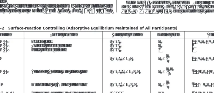
9. Solid-catalyzed reactions.Some Langmuir-Hinshelwood mechanisms for the reference reaction A +B →R +S (see also Tables 7.2, 7.3):
• Adsorption rate of A controlling:
ra= − =kPaθv
θv=1
/
1 + +KbPb+KrPr+KsPs+KlPl (1)Ke=PrPs/PaPb(equilibrium constant) lis an adsorbed substance that is chemically inert.
• Surface reaction rate controlling:
r =kPaPbθv2
θv= , summation over all substances absorbed (2)
• Reaction A2+B →R +S, with A2dissociated upon adsorption and with surface reaction rate controlling:
ra=kPaPbθv3
θv= (3)
• At constant Pand Tthe Piare eliminated in favor of niand the total pres- sure by:
Pa= P
Pi= P= P
+for products, RHS−for reactants, LHS V =
kt=
nana0 , for a Case (2) batch reaction (4)10. A continuously stirred tank reactor(CSTR) battery Material balances:
n′a0=n′a+ra1Vr1
n′a,j−⯗1=n′aj+rajVrj, for the jth stage For a first-order reaction, with ra=kCa:
=
=
for jtanks in series with the same temperatures and residence times ti= Vri/V′i, where V′is the volumetric flow rate.
11. Plug flow reactor(PFR):
rs= − =kCaαCbβ⋅ ⋅ ⋅
=k
α β
⋅ ⋅ ⋅ n′b
ᎏV′
n′a
ᎏV′
dn′a
ᎏdVr
ᎏ1 (1+kti)j
ᎏᎏᎏᎏ1 (1+k1t1)(1+k2t2)⋅ ⋅ ⋅(1+kjtj) Caj
ᎏCa0
dna
ᎏVPaPbθv2
ntRT ᎏP
ni0⫾(νi/νa)(na0−na) ᎏᎏᎏnt0+(∆ν/νa)(na0−na) ni
ᎏnt
na
ᎏnt
ᎏᎏᎏ1 (1+KaPa+KbPb+ ⋅ ⋅ ⋅) ᎏᎏ1
1+ KjPj
PrPs
ᎏPb
Ka
ᎏKe
dna
ᎏdt ᎏ1 V
7-4
RATE OF REACTION
The term rate of reactionmeans the rate of decomposition per unit volume,
ra= − , mol/(unit time) (unit volume) (7-1)
= , n0=na0(1 −xa) (7-2)
where xais the fractional conversion of substance A. A rate of forma- tion will have the opposite sign. The negative sign is required for the rate of decomposition to be a positive number. When the volume is constant,
ra= − only at constant volume (7-3) Law of Mass Action The effect of concentration on the rate is isolated as
ra=kf(Ca, Cb, . . .) (7-4) where the specific rate kis independent of concentration but does depend on temperature, catalysts, and other factors. The law of mass action states that the rate is proportional to the concentrations of the reactants. For the reaction
νaA+ νbB+ νcC+. . .⇒ νrR+ νsS+. . . (7-5) the rate equation is
ra= − =kCapCbqCcr. . . (7-6)
⇒ − at constant volume (7-7)
The exponents (p, q, r, . . .) are empirical, but they are identical with the stoichiometric coefficients (νa, νb, νc, . . .) when the stoichiometric equation truly represents the mechanism of reaction. The first group of exponents identifies the orderof the reaction, the stoichiometric coefficients the molecularity.
Effect of Temperature The Arrhenius equationrelates the spe- cific rate to the absolute temperature,
k =k0exp (7-8)
=exp
A − (7-9)ln k =A − (7-10)
Eis called the activation energy and k0the preexponential factor.
When presumably accurate data deviate from linearity as stated by the ᎏB
T ᎏB T ᎏ−E RT dCa
ᎏdt dna
ᎏdt ᎏ1 V dCa
ᎏdt dxa
ᎏdt na0
ᎏV dna
ᎏdt ᎏ1 V
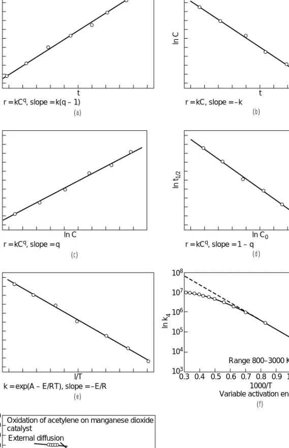
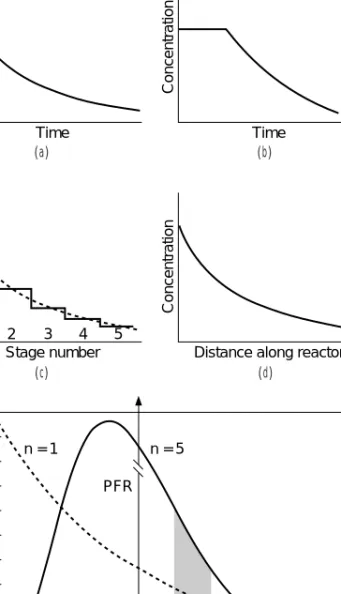
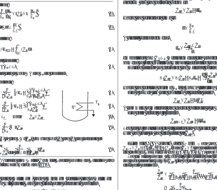
last equation, the reaction is believed to have a complex mechanism (Fig. 7-1g).
CONCENTRATION, MOLES, PARTIAL PRESSURE, AND MOLE FRACTION
Any property of a reacting system that changes regularly as the reac- tion proceeds can be formulated as a rate equation which should be convertible to the fundamental form in terms of concentration, Eq.
(7-4). Examples are the rates of change of electrical conductivity, of pH, or of optical rotation. The most common other variables are par- tial pressure piand mole fraction Ni. The relations between these units are
ni=VCi=ntNi= (7-11) where the subscript tdenotes the total mol and πthe total pressure.
For ideal gases, V =
ni= Ci= pi= pi= Ni (7-12) Other volume-explicit equations of state are sometimes required, such as the compressibility equation V =zRT/Por the truncated virial equation V=(1 +B′P)RT/P. The quantities zand B′are not constants, so some kind of averaging will be required. More accurate equations of state are even more difficult to use but are not often justified for kinetic work.
Designate δaas the increase in the total mol per mol decrease of substance A according to the stoichiometric equation Eq. (7-5):
δa= (7-13)
The total number of mols present is
nt=nt0+ δa(na0−na) =nt0+ δaxa=nt0+ δbxb=. . . (7-14) Accordingly,
− = δa = δb = δc =. . . (7-15) The various differentials are
dni=d(VCi) = d(Vpi) =d(ntNi) = dNi (7-16) The rate equation
ra= − dCa =kcCaα (7-17) ᎏdt
ᎏ1 V
nt
ᎏ1+ δiNi
ᎏ1 RT
dnc
ᎏdt dnb
ᎏdt dna
ᎏdt dnt
ᎏdt
(νr+ νs+ . . .)−(νa+ νb+ νc+. . .) ᎏᎏᎏᎏνa
ᎏπV RT ᎏV
RT ni
ᎏπ ntRT ᎏπ ntRT ᎏπ
ntpi
ᎏπ
RATE EQUATIONS
12. Material and energy balancesfor batch, CSTR, and PFR in Tables 7-5, 7-6, and 7-7.
13. Notation.A, B, R, S are participants in the reaction; the letters also are used to represent concentrations.
Ci=ni/Vror n′i/V′,concentration ni=mol of component iin the reactor n′i=molal flow rate of component i Vr=volume of reactor
V′ =volumetric flow rate νi=stoichiometric coefficient
ri=rate of reaction of substance i[mol/(unit time)(unit volume)]
α,β =empirical exponents in a rate equation TABLE 7-1 Basic Rate Equations(Concluded)
SOURCE: Adapted from Walas, Chemical Process Equipment Selection and Design,Butterworth-Heinemann, 1990.
t r = kCq, slope = k(q – 1)
l/Cq – 1
t r = kC, slope = –k
ln C
ln C r = kCq, slope = q
ln r
ln C0 r = kCq, slope = 1 – q ln t1/2
l/T k = exp(A – E/RT), slope = –E/R
ln k
0.3 0.4 0.5 0.6 0.7 0.8 1000/T Variable activation energy
0.9 1.0 1.1 1.2 1.3 Range 800–3000 K
ln k
108 107 106 105 104 103
10 12 14 16 18 20 10,000/T
22 24 26 28 30 Chemical rate
Pore diffusion External diffusion
Oxidation of acetylene on manganese dioxide catalyst
10 k
220 180 160 140 120 200
100 80 60 40 20
( a ) ( b )
( c ) ( d )
( f ) ( e )
6 4
FIG. 7-1 Constants of the power law and Arrhenius equations by linearization: (a) integrated equation, (b) integrated first order, (c) differential equation, (d) half-time method, (e) Arrhenius equation, (f) variable activation energy, and (g) change of mechanism with temperature (Tin K).
(a) (b)
(c) (d )
(e)
(f)
(g)
can be expressed in terms of pressure and mole fraction,
− =kc
α
paα (7-18)
or at constant volume,
− =kc α −1
paα=kppaα (7-19) where the specific rate in terms of partial pressure is
kp=kc α −1
(7-20) Typical Units of Specific Rates For order α, typical units are:
kc (L/g mol)α −1⋅s−1, and s−1when first order kp (g mol)/L⋅s⋅atmα
Furthermore,
− =kc
α
Naα
or
− =kc α −1
Naα
=kc α −1
Naα (7-21)
Various derivatives are evaluated in numerical Example 1.
Example 1: Rates of Change at Constant V or Constant P Consider the ideal gas reaction 2A ⇒B +2C occurring at 800°R, starting with 5 lb mol of pure A at 10 atm. The rate equation is
ra= − =700 Ca2lb mol/(ft3⋅h)
Evaluate the various rates of change at the time when the rate of reaction is ra= 0.1 lb mol/(ft3⋅h) and the reaction proceeds at (1) constant volume, and (2) con- stant pressure.
ra= − =700 Ca2=0.1 lb mol/(ft3⋅h)
Ca=
=0.01195 lb mol/ft3V0= = =291.6 ft3
Ca0= = =0.01715 lb mol/ft3 nt=0.5(3na0−na) lb mol
V= =29.16(15 −na) ft3 π = π0=3na0−naatm
At constant volume, na=V0Ca=291.6(0.01195) =3.4853 lb mol
=V0 = −291.6(0.1) = −29.16 lb mol/h
Na= =
= = (−29.16)
= −6.598 h−1
pa= atm
= =0.729(800)(−29.16) = −58.32 atm/h ᎏᎏ291.6
dna
ᎏdt ᎏRT
V0
dpa
ᎏdt naRT ᎏV0
ᎏᎏ6 5(3−3.4853/5)2 dna
ᎏdt ᎏᎏ6 na0(3−na/na0)2 dNa
ᎏdt
2na
ᎏ3na0−na
na
ᎏnt
dCa
ᎏdt dna
ᎏdt nt
ᎏnt0
(3na0−na) RT ᎏᎏ2π0
ᎏ5 291.6 na0
ᎏV0
5(0.729)(800) ᎏᎏ10 na0RT
ᎏπ0
ᎏ0.1 700 dna
ᎏdt ᎏ1 V
dna
ᎏdt ᎏ1 V
ᎏ1 1+ δaNa
ᎏπ RT
ᎏ1 1+ δaNa
nt
ᎏV dNa
ᎏdt
nt
ᎏV dNa
ᎏdt nt
ᎏᎏV(1+ δaNa) ᎏ1
RT ᎏ1 RT dpa
ᎏdt
ᎏ1 RT d(Vpa) ᎏdt ᎏ1 RTV
π = π0= π0=5
3 − atm= − =29.16 atm/h
At constant pressure, na=VCa=29.16(15 −na) (0.01195) =3.8768 lb mol
= −Vra= −324.4(0.1) = −32.44 lb mol/h
since V=29.16 (15 −3.8768) =324.4 ft3
Ca= = lb mol/ft3
=
=
(−32.44)
=0.1349 lb mol/(ft3⋅h)
= = (−32.44) = −7.8658 h−1
pa=Naπ0= atm
= = (−32.44) = −78.66 atm/h
V= ft3
=
− = (32.44) =945.95 ft3/h=
= − = − (−32.44) =6.488 h−1
SUMMARY
Rate At constant V At constant P
dnadt,lb mol/h −29.16 −32.44
dNa/dt,h−1 −6.598 −7.866
dpa/dt,atm/h −58.32 −78.66
dπ/dt,atm/h 29.16 0
dV/dt,ft3/h 0 946.0
dxa/dt,h−1 5.832 6.488
REACTION TIME IN FLOW REACTORS
Flow reactors usually operate at nearly constant pressure, and thus at variable density when there is a change of moles of gas or of tempera- ture. An apparent residence timeis the ratio of reactor volume and the inlet volumetric flow rate,
tapp= (7-22)
The true residence timeis obtained by integration of the rate equation,
t=
= = (7-23)The apparent time is readily evaluated and is popularly used to indi- cate the loading of a flow reactor.
A related concept is that of space velocity,which is a ratio of a flow rate at STP (usually 60°F, 1 atm) to the size of the reactor. The most common versions in typical units are:
GHSV (gas hourly space velocity) =(volumes of feed as gas at STP/h)/(volume of reactor or its content of catalyst) =SCFH gas feed/ft3.
LHSV (liquid hourly space velocity) =(volume of liquid feed at 60°F/h)/(ft3of reactor) =SCFH liquid feed/ft3.
WHSV (weight hourly space velocity) =(lb feed/h)/(lb catalyst).
It is usually advisable to spell out the units when the acronym is used, since the units are arbitrary.
ᎏᎏdn kV′(n/V′)q ᎏV′rdn
dVr
ᎏV′
Vr
ᎏV′0
ᎏ1 5 dna
ᎏdt ᎏ1 na0
na0−na
ᎏna0
ᎏd dt dxa
ᎏdt
0.729(800) ᎏᎏ20 dna
ᎏdt ᎏ2πRT0
ᎏdV dt
(3na0−na)RT ᎏᎏ2π0
(6)(10)(5) ᎏᎏ(15−3.8768)2 dna
ᎏdt 6π0
ᎏᎏ(3na0−na)2 dpa
ᎏdt
2π0na
ᎏ3na0−na
ᎏᎏ30 (15−3.8768)2 dna
ᎏdt 6na0
ᎏᎏ(3na0−na)2 dNa
ᎏdt
ᎏᎏ15 (15−3.8768)2 ᎏ1
29.16 dna
ᎏdt ᎏᎏ15
(15−na)2 ᎏ1 29.16 dCa
ᎏdt
na
ᎏᎏ29.16(15−na) na
ᎏV dna
ᎏdt
dna
ᎏdt ᎏ5 na0
ᎏdπ dt
na
ᎏna0
3na0−na
ᎏᎏ2na0
nt
ᎏnt0
CONSTANTS OF THE RATE EQUATION
The problem is to apply experimental data to find the constants of assumed rate equations, of which some of the simpler examples are:
r = − =kCq (7-24)
or r = − =exp
a− Cq (7-25)or ra= − =kCapCb
q (7-26)
Experimental data that are most easily obtained are of (C, t), (p, t), (r, t), or (C, T, t). Values of the rate are obtainable directly from mea- surements on a continuous stirred tank reactor (CSTR), or they may be obtained from (C, t) data by numerical means, usually by first curve fitting and then differentiating. When other properties are measured to follow the course of reaction—say, conductivity—those measure- ments are best converted to concentrations before kinetic analysis is started.
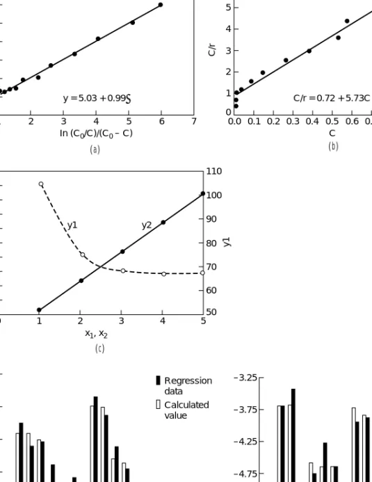
The most common ways of evaluating the constants are from linear rearrangements of the rate equations or their integrals. Figure 7-1 examines power law and Arrhenius equations, and Fig. 7-2 has some more complex cases.
From the Differential Equation Linear regression can be applied with the differential equation to obtain constants. Taking log- arithms of Eq. (7-25),
ln r =a − +qln C (7-27)
The variables that are combined linearly are ln r,1/T,and ln C.Multi- linear regression software can be used to find the constants, or only three sets of the data suitably spaced can be used and the constants found by simultaneous solution of three linear equations. For a lin- earized Eq. (7-26) the variables are logarithms of r, Ca, and Cb. The logarithmic form of Eq. (7-24) has only two constants, so the data can be plotted and the constants read off the slope and intercept of the best straight line.
From the Integrated Equation The integral of Eq. (7-24) is
k= ln , whenq=1 (7-28)
q−1
−1
, whenq≠1 (7-29)A value of qis assumed and values of kare calculated for each data point. The correct value of qhas been chosen when the values of kare nearly constant or show no drift. This procedure is applicable for a rate equation of any complexity if it can be integrated. Eqs. (7-28) and (7-29) can also be put into linear form:
ln =k(t −t0), whenq=1 (7-30)
q−1
= q−1+k(q−1) (t −t0), whenq≠1 (7-31) When the plots are collinear, the correct value of kis found from the slope of the best straight line.
From Half-Times The time by which one-half of the reactant has been converted is called the half-time.From Eq. (7-24),
kt1/2=ln 2, q=1
q≠1 (7-32)
When several sets of (C0, t1/2) are known, values of qare tried until one is found that makes all kvalues substantially the same. Alternatively, the constants may be found from a linearized plot,
ln t1/2=ln 2q−1−1+(1 −q) ln C0 (7-33) ᎏ(q−1)k
2q−1−1 ᎏᎏ(q−1)C0q−1 ᎏ1
C0
ᎏ1 C
C0
ᎏC
C0
ᎏC C0
q−1
ᎏᎏ(t−t0) (q−1) C0
ᎏC ᎏ1 t−t0
ᎏb T dCa
ᎏdt
ᎏb t ᎏdC
dt ᎏdC
dt
Complex Rate Equations Complex rate equations may require individual treatment, although the examples in Fig. 7-2 are all lin- earizable. A perfectly general procedure is nonlinear regression. For instance, when r =f(C, a, b, . . .) where (a, b, . . .) are the constants to be found, the condition is
[ri−f(Ci, a, b, . . .)]2⇒Minimum (7-34)
and = =. . .=0 (7-35)
Much professional software is devoted to this problem. A diskette for sets of differential and algebraic equations with parameters to be found by this method is by Constantinides (Applied Numerical Meth- ods with Personal Computers,McGraw-Hill, 1987).
The acquisition of kinetic data and parameter esti