Regional Income, Household Expenditure, Poverty, and Education Convergence Clubs at the District Level in Indonesia

(1)

121

Regional Income, Household Expenditure, Poverty, and Education Convergence Clubs at the District Level in Indonesia

Muhammad Zulfiqar Firdaus

Faculty of Economics and Business, Universitas Indonesia.

Gedung Dekanat FEB UI Kampus Widjojo Nitisastro, Jl. Prof. DR. Sumitro Djojohadikusumo, Kukusan, Kecamatan Beji, Kota Depok, Jawa Barat 16424, Indonesia

Correspondence: [email protected]

Received: April 22, 2023; Revised: May 18, 2023; Accepted: September 5, 2023 Permalink/DOI: http://dx.doi.org/10.17977/um002v15i22023p121

Abstract

This article reinvestigates the regional convergence in GDP per capita, household expenditure per capita, poverty rate, and average years of schooling in Indonesia at the district level during 2000–2017 using the convergence club method. This article finds that regional inequality in Indonesia at the district level is characterized by two convergence clubs in GDP per capita, five convergence clubs in household expenditure per capita, six convergence clubs in poverty, and five convergence clubs in average years of schooling. This article also confirms the existence of spatial concentration among regions and a development gap between the west and east sides of Indonesia.

Keywords: Convergence, Regional Inequality, Development.

JEL classification: H54, R11, R58

INTRODUCTION

Regional inequality within countries has become one of the major interests among economists and policymakers in recent years (Lessman & Seidel, 2017). Regional inequality may harm a country since it could reduce economic efficiency (Holmes &

Mayhew, 2015), exacerbate social tension (Case & Deaton, 2020), increase resentment toward urban elites (Rodriguez-Pose, 2018), lead to conflict (Floerkemeier et al., 2021), and trap poorer regions in a low-productivity and low-income equilibrium (Corvers &

Mayhew, 2021). As the largest archipelago in the world, Indonesia is characterized by regional inequality in terms of different levels of development, resource endowments, population distributions, and ethnicity among its regions, which has become a major issue (Vidyattama, 2013). Furthermore, the decentralization process of Indonesia, which was carried out without much preparation in terms of intuitional capacity and local authority qualifications, has heightened concerns about regional inequality (Brodjonegoro, 2004; Nasution, 2016).

Motivated by these facts, this article intends to reinvestigate the evolution of regional inequality and the possibility of convergence across 514 districts of Indonesia during 2000–2017 in terms of regional income, household expenditure per-capita, poverty, and average years of schooling. This study contributes to the regional convergence literature in two aspects. First, this article examines the convergence clubs (Philips & Sul, 2007; 2009) of four development indicators, which are GDP per capita,

(2)

122

household expenditure per capita, poverty rate, and average years of schooling. Second, from a methodological point of view, this article evaluates the previous club convergence study written by Aginta et al. (2021) and provides a possible alternative to overcome data limitations in conducting regional convergence studies in Indonesia as it uses an alternative data imputation method.

In brief, this article finds that there is no global/full panel convergence in GDP per capita, household expenditure per capita, poverty, and average years of schooling during 2000–2017. Regional inequality in Indonesia at the district level is characterized by two convergence clubs in GDP per capita, five convergence clubs in household expenditure per capita, six convergence clubs in poverty, and five convergence clubs in average years of schooling. Furthermore, this article confirms the existence of spatial concentration across regions and a development gap between the east and west sides of Indonesia in terms of household expenditure per capita, poverty, and average years of schooling.

LITERATURE REVIEW

Convergence studies are typically carried out using classical methods such as beta (β) convergence and sigma (σ) convergence. The basic premise of beta convergence is that the growth of poor regions would be faster than the growth of rich regions because of their higher capital marginal productivity, assuming equal saving rates and diminishing returns on marginal productivity of capital. Beta convergence can take two different forms, which are conditional and unconditional/absolute. Conditional beta convergence includes factors that predict the convergence process, while unconditional/absolute beta convergence excludes control variables that impact the convergence process. However, because beta convergence may not always imply a reduction in inequality, sigma convergence, which implies a reduction in dispersion overtime, must be evaluated and analysed in addition to beta convergence. For this reason, these two concepts are usually used together in analysis, where beta convergence is required but insufficient for the occurrence of sigma convergence.

Aside from these two types of convergence, there is also a club convergence method, which highlights the importance of multiple equilibria and heterogeneity. This is theoretically important because the method might capture the persistent differences in endowments, preferences, and technologies among regions, while the classical convergence methods only capture the average behaviour and common long-run equilibrium. In other words, under the club convergence method, regions may be divided into multiple convergence clubs rather than seamlessly converging toward a single long-run equilibrium.

Many researchers in Indonesia have carried out regional convergence studies using a variety of methods (see Table 1). Garcia and Soelistianingsih (1998) study the GDP per capita convergence of 26 provinces between 1975-1993. The results indicate that absolute and conditional beta convergence exist where conditional beta convergence has a higher speed of convergence. Furthermore, their study finds that oil and gas variables as well as educational coverage increase the speed of convergence. In extending the study using the extended data set, Hill et al. (2008) conduct a study and find that absolute and conditional beta convergence existed during the period from 1975 to 2004. In addition, their study finds that the mining sector slows the speed of convergence. Tirtosuharto (2013) implements sigma convergence and beta convergence to test the convergence of 26 provinces during the period of 1997 to 2012. The study

(3)

123

finds that there was no sigma convergence from 1997 to 2012. Meanwhile, absolute beta convergence occurred between 1997 and 2000, and not between 2001 and 2012.

Kharisma and Saleh (2013) investigate sigma convergence, as well as absolute and conditional beta convergence, using an extended dataset. Their study shows that sigma convergence occurred between 1984 and 1996, but not between 1997 and 1998;

and sigma convergence exhibited considerable fluctuations between 1999 and 2008.

Furthermore, their study finds that the degree of openness and educational attainment are the most crucial conditional factors in affecting convergence. Vidyattama (2013) employs the models of spatial autoregressive (SAR) and spatial error (SEM) in examining the neighbourhood effects. As indicators, he looks at GDP per capita and the Human Development Index of 26 provinces and 294 districts. His study concludes that the neighbourhood impact is minor but statistically insignificant after building an inverted distance matrix.

Kurniawan et al. (2019) use the club convergence method to assess a few economic and social indicators at the provincial level. To obtain a fully balanced panel dataset, missing observations in the data set are interpolated. The study finds that there are 2 convergence clubs for all variables. Mendez and Kataoka (2021) also use the club convergence method to look at the evolution of regional inequalities in labor productivity, capital accumulation, and efficiency in 26 provinces during 1990-2010.

The results suggest that labor productivity, physical capital, and human capital are all characterized by 2, 4, and 2 convergence clubs, respectively. In addition, a unique convergence club for aggregate efficiency is discovered. Aginta et al. (2021) use a district-level dataset to assess the convergence of GDP per capita during 2000-2017.

Their findings reveal 5 convergence clubs among 514 districts, with the wealthiest club characterized by metropolitan cities and natural resource-rich districts, while the poorest group of districts are primarily found on the east side of Indonesia.

(4)

124 Table 1. Regional convergence studies in Indonesia

Writer(s) Indicator(s) Data Methods Results

Garcia &

Soelistianingsih (1998)

GDP per capita 26 Provinces:

1975-1993

Absolute and conditional β convergence

- β convergence exists and conditional β convergence accelerates the speed of convergence

- Positive relationship between convergence and oil & gas variables - Positive relationship between convergence and educational coverage Hill et al. (2008) - GDP per capita

- GDP per capita non-mining

26 Provinces:

1975-2004

Absolute and conditional β convergence

- Absolute and conditional β convergence exists

- The speed of convergence is declining overtime as the mining sector declines

Tirtosuharto (2013) GDP per capita 26 Provinces:

1997-2012

- σ convergence

- Absolute β convergence

- There is no σ convergence

- Absolute β convergence occurred between 1997 and 2000, but not between 2001 and 2012

Kharisma & Saleh (2013)

1984-2008

- σ convergence

- Absolute and conditional β convergence

- σ convergence occurred between 1984 and 1996, not occurred in 1997-1998, and varied during 1999-2008

- Absolute and conditional β convergence exists

- The most important conditional factors are the degree of openness and educational attainment.

Vidyattama (2013) - GDP per capita - Human

Development Index (HDI)

26 Provinces &

294 Districts:

1999-2008

- Absolute β convergence - Spatial autoregressive lag and spatial error models

- There is no absolute β convergence with spatial analysis for GDP per capita at provincial and district level

- There is no absolute β convergence with spatial analysis for HDI at provincial and district level

Kurniawan et al.

(2019)

- GDP per capita - Gini coefficient - School enrolment - Fertility rate

33 Provinces:

1969-2013

Club convergence - 2 convergences clubs - Spatial heterogeneity

Mendez & Kataoka (2021)

- Labor productivity - Physical capital - Human capital - Efficiency

26 Provinces:

1990-2010

Club convergence - 2 labor productivity convergence clubs - 4 physical capital convergence clubs - 2 human capital convergence clubs - Unique convergence for efficiency

(5)

125 Aginta et al. (2021) GDP per capita 514 Districts:

2000-2017

Club convergence - 5 convergence clubs

- Gap in development between west and east side of Indonesia Gunawan et al.

(2021)

2001-2017

- Club convergence - Ordered logit regression

- 4 convergence clubs

- Labor share and labor productivity increase the likelihood of provinces moving to the higher level of convergence club Mendez (2020) - Overall efficiency

- Pure efficiency - Scale efficiency

26 Provinces:

1990-2010

Classical and distributional convergence

- 2 convergence clubs for overall and pure efficiency - 1 convergence clubs for scale efficiency

Santoz-Marquez et al. (2021)

GDP per capita 34 Provinces &

514 Districts:

2001-2017

- Distributional convergence - Getis filter

- Lack of distributional convergence

- The indication that spatial dependence could be helpful in reducing extreme disparities

Miranti (2021) Poverty indicators (P0, P1, P2)

514 Districts:

2010-2018

- Distributional convergence

- Spatial convergence

- Distributional and spatial convergence take place in all three poverty indicators

- Overall clustering pattern and a persistent West–East polarization in poverty indicators convergence

- Spatial effect is significantly low in accelerating convergence rates in poverty reduction

Source: Author’s documentation

(6)

126

Using the classical and distributional convergence methods, Mendez (2020) examines the convergence of regional efficiency among 26 provinces from 1990 to 2010, focusing on 3 constructed metrics: overall efficiency, pure efficiency, and scale efficiency. All of the metrics indicate the presence of convergence under the classical convergence methods. The results of the distributional convergence method, on the other hand, reveal 2 convergence clubs in terms of overall and pure efficiency. In examining the convergence of regional incomes per capita using datasets of provinces and districts during 2000–2017, Santos-Marquez et al. (2021) use a distributional convergence method with Getis spatial filtering. The study reveals that spatial autocorrelation is only significant and robust at the district level. Furthermore, their findings suggest that spatial effects could be important in the convergence process.

Lastly, Miranti (2021) uses the distributional convergence and spatial convergence methods in evaluating the convergence of poverty among 514 districts from 2010–2018.

The study finds that distributional and spatial convergence exist for 3 poverty indicators. In the convergence of poverty indicators, there is also an overall clustering tendency and a longstanding West–East polarization. Furthermore, the study finds that spatial effects could slightly accelerate the convergence process.

METHOD

Classical Convergence: Beta and Sigma

To capture and explain some of the stylised facts regarding GDP per capita, household expenditure, poverty, and average years of schooling explained in Section 5, this article uses classical convergence methods, which are absolute beta (β) convergence and sigma (σ) convergence. Following the concept introduced by Barro and Sala-i- Martin (1992), absolute beta convergence can be modelled as follows:

(¹

𝑇) . 𝑙𝑛^𝑦^𝑖𝑇

𝑦_𝑖0 = 𝛼 −^(1−𝑒^−𝛽𝑇⁾

𝑇 . (𝑦_𝑖0) + 𝑤_𝑖,0𝑇 (1) where y represents an analysed variable, i represents a region (district), T and 0 are the latest period and the first period of observed data, β is known as the speed of convergence, α represents unobserved parameters including the steady-state value, and 𝑤_𝑖,0𝑇 is the error term. The first term on the left side (¹

𝑇) . 𝑙𝑛^𝑦^𝑖𝑇

𝑦_𝑖0, represents the growth of the analysed variable, which means equation (1) can also be written in a simplified regression equation as follows:

𝐺𝑟𝑜𝑤𝑡ℎ 𝑜𝑓 𝑦_𝑖 = 𝛼₀+ 𝛼₁𝑦_𝑖(𝑡₀) + 𝑣_𝑖 (2)

when the estimated parameter of the analysed variable's first period 𝛼₁ in equation (2) has a negative relationship with the growth of the analysed variable, it means the absolute beta convergence exists. Furthermore, when the absolute beta convergence exists, we can solve for β and estimate a “half-life” parameter, which represents the estimated time required for the inequality to be halved by the following equation:

ℎ𝑎𝑙𝑓 𝑙𝑖𝑓𝑒 = ^{𝑙𝑜𝑔2}

𝛽 (3)

(7)

127

Meanwhile, sigma convergence, which implies a reduction in the dispersion of the analysed variable, can be analysed by calculating the standard deviation of the analysed variable for each year (Barro & Sala-i-Martin, 2004, p. 462), using the formula as follows:

𝑆_𝑡 = √¹

𝑛∑ (𝑦^𝑛_𝑖 _𝑖𝑡 − 𝑦 _𝑡)² (4)

where 𝑆_𝑡 represents the standard deviation of the analysed variable at period t, 𝑦_𝑖𝑡 and 𝑦 _𝑡 represent the analysed variable of district i at period t and the average of the analysed variable at period t respectively, and n represents the number of districts. If there is a reduction in the standard deviation overtime, for instance when 𝑆_𝑡+1 is less than 𝑆_𝑡, it means the sigma convergence exists.

Club Convergence

In order to identify the convergence clubs, this article uses the club convergence method introduced by Phillips and Sul (2007, 2009). The method has three advantages compared to the classical convergence methods. First, it takes into account individual differences and changes in behaviour. Second, it does not rely on trend stationarity or random non-stationarity assumptions. Third, it allows for the grouping of similar transition paths in individual behaviour. The method requires us to decompose the panel data set of the analysed variable into the following form:

𝑦_𝑖𝑡 = Ω_𝑖𝑡+ 𝜌_𝑖𝑡 (5)

where Ω_𝑖𝑡 denotes permanent common components and 𝜌_𝑖𝑡 represents a transitory component. Equation (5) is then transformed into a dynamic factor form as follows:

𝑦_𝑖𝑡 = (^Ω^𝑖𝑡^+𝜌^𝑖𝑡

µ_𝑡 ) µ_𝑡= δ_𝑖𝑡µ_𝑡 (6)

where δ_𝑖𝑡 is a time-variant heterogenous component, which represents the heterogenous proximity between 𝑦_𝑖𝑡 and common component µ_𝑡. In eliminating Ω_𝑖𝑡 and measuring the transition parameter δ_𝑖𝑡 in equation (6), a relative transition parameter 𝑟_𝑖𝑡 is proposed as follows:

𝑟_𝑖𝑡 = 1 ^𝑦^𝑖𝑡

𝑁∑^𝑁_𝑖=1𝑦_𝑖𝑡= 1 ^δ^𝑖𝑡

𝑁∑^𝑁_𝑖=1δ_𝑖𝑡 (7)

Equation (7) compares individual economic behaviours to the regional system's average performance relatively. In this case, the existence of convergence is defined when t ∞, and 𝑟_𝑖𝑡 1, where the cross-sectional variance of 𝑟_𝑖𝑡, 𝑅_𝑡= 𝑁⁻¹∑ (𝑟_𝑖 _𝑖𝑡− 1)², converges to zero. When convergence does not occur, a variety of outcomes are possible. The proposed log t-test will reject the convergence hypothesis if 𝑅_𝑡 does not change or consistently increases. The operationalized form of the previously explained convergence test is given by:

𝑙𝑜𝑔(^𝑅¹

𝑅𝑡) − 2𝑙𝑜𝑔 (𝑙𝑜𝑔𝑡) = 𝑎 + 𝑏 log(𝑡) + 𝑣_𝑡 (8)

(8)

128

If 𝑏 in equation (8) is greater than 0 and statistically significant, we can conclude that the entire sample converges (there is a global/full panel convergence). On the other hand, when b is less than 0 and t-statistic of 𝑏 is less than -1.65, we can reject the convergence hypothesis. “When the convergence hypothesis is rejected, the sample can be utilized to identify local convergence clubs” (Phillips & Sul 2007; 2009; Du 2017).

The steps in identifying local clubs of convergence (also known as clustering algorithm) are summarized in the next sub-section. Furthermore, 𝑏 coefficient also can imply 3 different types of convergence. First, when 𝑏 < 0, it implies that the divergence occurs.

Second, when 0 ≤ 𝑏 < 2, it implies that there is relative convergence of growth rates.

Third, when b ≥2, it implies that there is absolute convergence (convergence in levels).

Lastly, the speed of convergence can also be calculated as ^𝑏

2 (𝑏 divided by two), when the convergence occurs.

Clustering Algorithm

The data clustering algorithm introduced by Phillips and Sul (2009) is summarized as follows:

• 1^st step: According to their observation in the last period, sample units (districts) are ordered in descending order.

• 2^nd step: An initial club of districts (Gk) is generated by pooling the first two districts. The next district is added to the club and verified whether the log t-test indicates convergence (t-statistic is greater than -1.65). As long as the convergence exists, the next districts can keep being added to the initial club.

• 3^rd step: A complementary initial club (Gc) is generated by the districts that are not members of the initial club. Each district from this complementary initial club (Gc) is added to the initial club (Gk) and tested using the log t-test. A new initial club is generated by the district if the t-statistic from the log t-test is greater than zero.

• 4^th step: The log t-test is conducted for the districts that were not selected in the third step. These districts generate a new initial club if their t-statistic from the log t-test is greater than -1.65. If not, the first up until the third step are repeated for these districts. If there is no initial club that is identified, these districts are considered divergent and the algorithm is stopped.

• 5^th step: All of the identified initial clubs will be pooled together and tested to check whether they can be combined/merged together. If t-statistic from the log t-test is greater than -1.65, the clubs can be combined together to generate a new club.

Data

This article uses a constructed data set which consists the data of annual GDP per capita, household expenditure per capita, poverty rate (percentage of poor/P0), and average years of schooling of 514 districts from 2000 to 2017. The data of annual GDP per capita, household expenditure per capita, poverty rate, and average years of schooling are obtained from World Bank INDO-DAPOER (Indonesia Database for Policy and Economic Research). The data of annual GDP per capita is constructed by dividing regional GDP data with population data. It is important to note that the club convergence method requires a balanced panel data set without gaps. Since Indonesia experienced district proliferation during 2000-2017 which causes some missing observations in original data, the constructed data set must be imputed to accommodate the missing observations caused by district proliferation.

(9)

129

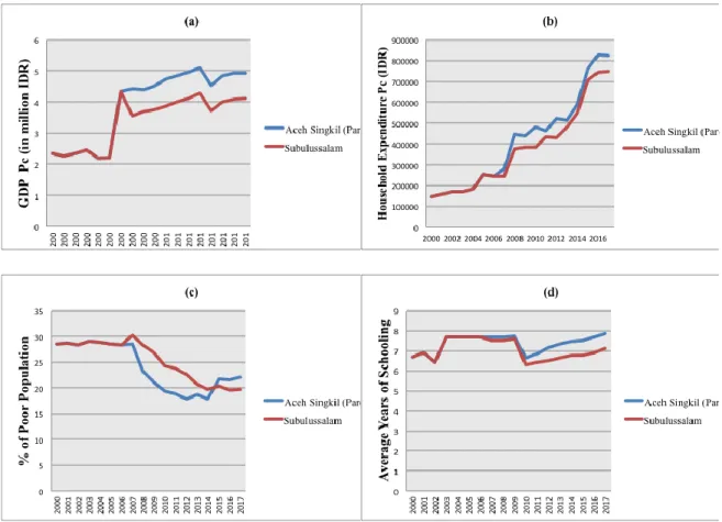
In contrast with the data imputation method used by previous study (i.e. Aginta et al., 2021), the data of GDP per capita, household expenditure per capita, poverty rate, and average years of schooling in this study are imputed using the assumption that split districts follow their parent districts' data before they split. In other words, the data of parent districts is used to fill in the missing observations in new districts before they split. Figure 1 illustrates the assumption used for filling in the missing observations in new districts. Panel (a) – (d) illustrates the imputed data of GDP per capita, household expenditure, poverty rate and average years of schooling respectively. Furthermore, because some of the parent districts' observations are also missing, particularly in 2000–

2001, this article uses linear regression based on the subsequent and/or proceeding period observations to impute the missing observations in the parent districts. Because measurement errors resulting from data imputation are unavoidable, a robustness check for data imputation is carried out (see Appendix 1).

Figure 1. Data imputation illustration

Note: Subulussalam split from its parent (Aceh Singkil) in 2007, therefore Subulussalam data follows its parent data before 2007 Source: INDO-DAPOER, Author’s calculation

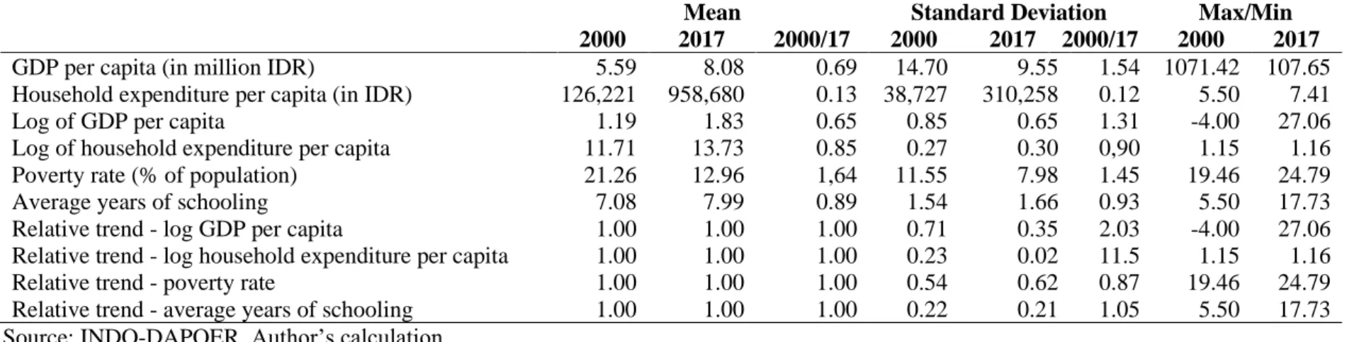
Table 2 presents the descriptive statistics of the constructed data set. For the purpose of analysis as well as to fulfil the methodology’s requirements, GDP per capita and household expenditure per capita are transformed into the log form. Furthermore, the relative trend of variables is also calculated by dividing the data (variables) with their average for each year for the purpose of analysing the transition paths. In addition, similar to the study conducted by Phillips and Sul (2007), this study uses the Hodrick- Prescott (HP) filter with a smoothing parameter (λ) of 400 in isolating the cyclical component from the variables’ trend.

(10)

130

Table 2. Descriptive statistics

Mean Standard Deviation Max/Min

2000 2017 2000/17 2000 2017 2000/17 2000 2017

GDP per capita (in million IDR) 5.59 8.08 0.69 14.70 9.55 1.54 1071.42 107.65

Household expenditure per capita (in IDR) 126,221 958,680 0.13 38,727 310,258 0.12 5.50 7.41

Log of GDP per capita 1.19 1.83 0.65 0.85 0.65 1.31 -4.00 27.06

Log of household expenditure per capita 11.71 13.73 0.85 0.27 0.30 0,90 1.15 1.16

Poverty rate (% of population) 21.26 12.96 1,64 11.55 7.98 1.45 19.46 24.79

Average years of schooling 7.08 7.99 0.89 1.54 1.66 0.93 5.50 17.73

Relative trend - log GDP per capita 1.00 1.00 1.00 0.71 0.35 2.03 -4.00 27.06

Relative trend - log household expenditure per capita 1.00 1.00 1.00 0.23 0.02 11.5 1.15 1.16

Relative trend - poverty rate 1.00 1.00 1.00 0.54 0.62 0.87 19.46 24.79

Relative trend - average years of schooling 1.00 1.00 1.00 0.22 0.21 1.05 5.50 17.73 Source: INDO-DAPOER, Author’s calculation

(11)

131

RESULTS AND DISCUSSION Stylised Facts

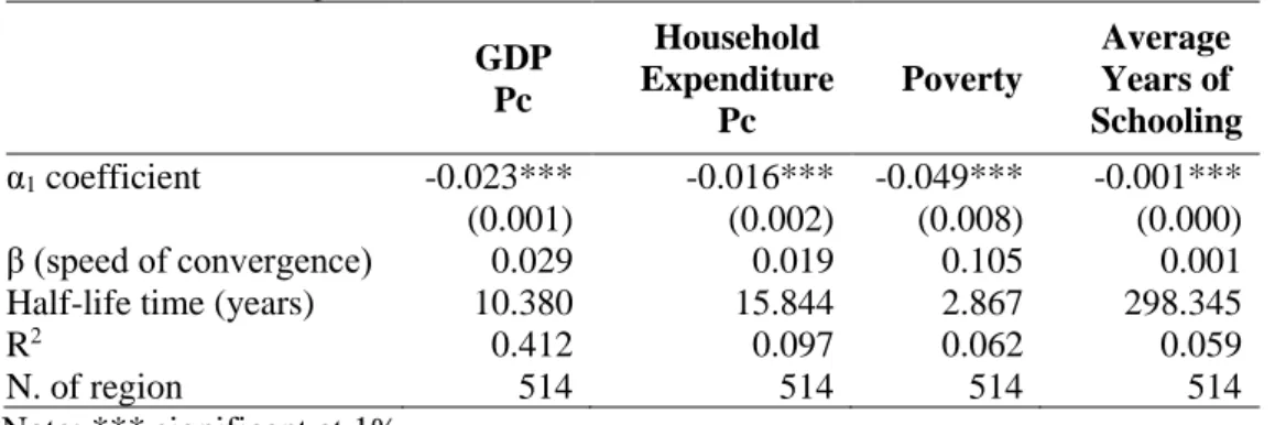
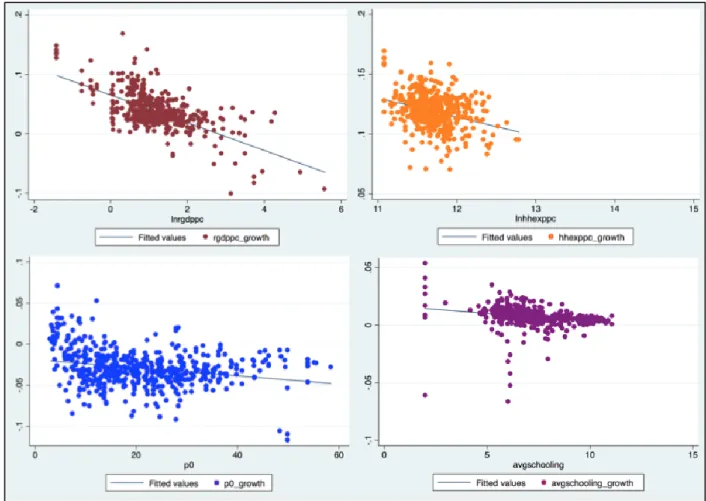
In explaining the evolution of regional inequality in Indonesia from 2000 to 2017, this study uses absolute beta and sigma converge methods. First, recalling the regression equation (2), Table 3 and Figure 2 summarize and plot the results of the absolute beta convergence test, respectively. From the table, since the α1 coefficient is negative and statistically significant for all variables, we can say that absolute beta convergence in GDP per capita, household expenditure per capita, poverty rate, and average years of schooling exists among districts during 2000-2017. The speed of convergence and half- life time suggest that the reduction in poverty’s inequality is the fastest, with a 10.5%

reduction per year, and the observed inequality would be halved in just two years, which is then followed by GDP per capita, household expenditure per capita, and average years of schooling, respectively. It is also important to notice that the reduction in inequality of average years of schooling is estimated to be very slow compared to other variables’ inequality, at only 0.1% per year.

Table 3. Beta convergence results

GDP Pc

Household Expenditure

Pc

Poverty

Average Years of Schooling α1 coefficient -0.023*** -0.016*** -0.049*** -0.001***

(0.001) (0.002) (0.008) (0.000)

β (speed of convergence) 0.029 0.019 0.105 0.001

Half-life time (years) 10.380 15.844 2.867 298.345

R² 0.412 0.097 0.062 0.059

N. of region 514 514 514 514

Note: *** significant at 1%.

Source: Author’s calculation

(12)

132

Figure 2. Regional disparities evolution-Beta convergence approach Source: Author’s calculation

Note: A beta convergence test using 342 parent districts is performed for the robustness check of data imputation results. The results are not significantly different from the results of using 514 districts (see Appendix 1).

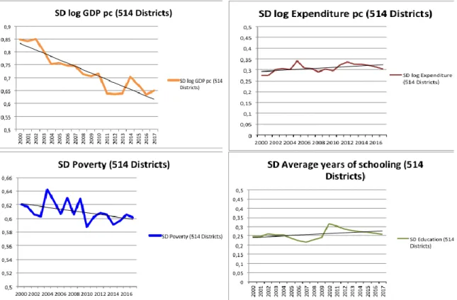
Second, using the sigma convergence approach, which is plotted in Figure 3, we can say that sigma convergence in GDP per capita among districts in Indonesia existed during 2000–2017, as the standard deviation trend line of GDP per capita shows a declining trend over time. Similarly, the standard deviation linear trend line of poverty suggests that sigma convergence in poverty exists. On the other hand, the standard deviation’s linear trend line of household expenditure per capita and average years of schooling implies that there is no sigma convergence in household expenditure per capita and average years of schooling.

(13)

133

Figure 3. Regional disparities evolution-Sigma convergence approach

Note: A sigma convergence test using 342 parent districts is performed for the robustness check of data imputation results.The results are not significantly different from the results of using 514 districts (see Appendix 1). Source: Author’s calculation

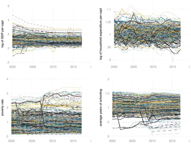
In addition to the absolute beta and sigma convergence, Figure 4 plots the relative trend of each variable, which shows the actual dynamics of all districts. The figure suggests that the convergence process in GDP per capita and household expenditure per capita has not only happened because poorer districts have grown faster, but also because richer districts had negative growth during 2000-2017 in terms of these two variables at some point. Similarly, the convergence process in poverty and average years of schooling has also happened, not only because some of the districts with higher growth in poverty and lower growth in average years of schooling have slowed down, but also because some of the districts with lower growth in poverty and higher growth in average years of schooling have grown faster at some point.

(14)

134

Figure 4. Regional disparities evolution-Relative trend approach Source: Author’s calculation

Convergence Clubs

The identification of convergence clubs in GDP per capita, household expenditure per capita, poverty and average years of schooling is summarized in Table 4. The log t- test results of GDP per capita, household expenditure per capita, poverty, and average years of schooling of 514 Indonesian districts during 2000–2017 suggest that we can reject the hypothesis of global (full panel) convergence at the 1% significance level, since the b coefficient is significantly less than 0 and t-statistic of b is below -1.65 for all variables. This means that all variables do not converge into a single long-run equilibrium.

(15)

135 Table 4. Convergence clubs

(1) (2) (3) (4) (5) (6)

GDP per-capita

Initial clubs [No. members] b (t-stat of b) Merging Test Final clubs [No. members] Average 2000 Average 2017

Total sample [514 districts] -0.241*** (-36.250)

Club 1 [337 districts] -0.020 (-1.449) Club 1+2 -0.241*** (-36.250) Club 1 [337 districts] Rp. 6.139 mio Rp. 9.719 mio

Club 2 [117 districts] 0.160 (4.649) Club 2 [117 districts] Rp. 4.571 mio Rp. 4.972 mio

Expenditure per-capita

Total sample [514 districts] -0.842*** (-95.515)

Club 1 [71 districts] 0.317 (3.804) Club 1+2 -0.024 (-0.434) Club 1 [173 districts] Rp. 142,903 Rp. 1,252,356 Club 2 [102 districts] 0.085 (1.315) Club 2+3 -0.113***(-1.945) Club 2 [205 districts] Rp. 122,406 Rp. 884,5535 Club 3 [72 districts] 0.124 (1.457) Club 3+4 0.057 (0.729) Club 3 [116 districts] Rp. 112,889 Rp. 723,421 Club 4 [133 district] 0.172 (1.870) Club 4+5 -0.125***(-2.087) Club 4 [18 districts] Rp. 99,092 Rp. 563,768 Club 5 [88 districts] 0.124 (1.793) Club 5+6 0.131 (1.712) Club 5 [2 districts] Rp. 91,587 Rp. 354,812

Club 6 [17 districts] 0.283 (2.260) Club 6+7 0.167(1.579)

Club 7 [11 districts] 0.065 (0.938) Club 7+8 -0.024 (-0.341)

Club 8 [10 districts] 0.387 (3.149) Club 8+9 0.401(3.565)

Club 9 [5 districts] 0.864 (8.705) Club 9+10 -1.282***(-10.973) Club 10 [3 districts] 0.059 (3.459) Club 10+11 -0.568*** (-3.782)

Club 11 [2 districts] 3.603 (2.222)

(16)

136 Poverty rate

Total sample [514 districts] -1.231***(-58.385)

Club 1 [6 districts] 0.382 (4.628) Club 1+2 0.494 (6.089) Club 1 [38 districts] 39.46% 33.10%

Club 3 [26 districts] 0.309 (4.749) Club 3+4 -0.277***(-7.408) Club 3 [125 districts] 25.07% 15.31%

Club 4 [34 districts] 0.427 (3.830) Club 4+5 0.256(2.991) Club 4 [112 districts] 18.92% 10.78%

Club 6 [125 districts] 0.129 (1.864) Club 6+7 -0.195***(-4.058) Club 6 [7 districts] 14.44% 3.49%

Club 7 [112 districts] 0.429 (3.641) Club 7+8 -0.472*** (-20.383) Club 8 [177 districts] -0.065 (-1.274) Club 8+9 -0.238*** (-5.584)

Club 9 [7 districts] -0.085 (-0.732)

Average years of schooling

Total sample [514 districts] -0.971***(-538.883)

Club 1 [42 districts] 0.843 (7.584) Club 1+2 -0.030 (-0.706) Club 1 [159 districts] 8.39 years 9.77 years Club 2 [117 districts] 0.036 (0.649) Club 2+3 -0.476*** (-22.539) Club 2 [214 districts] 6.87 years 7.82 years Club 3 [214 districts] 0.092 (2.045) Club 3+4 -0.556*** (-68.489) Club 3 [124 districts] 6.11 years 6.65 years Club 4 [124 districts] -0.048 (-1.097) Club 4+5 -0.579*** (-58.228) Club 4 [10 districts] 4.66 years 4.22 years Club 5 [10 districts] 0.655 (7.053) Club 5+6 -0.336*** (-5.627) Club 5 [5 districts] 4.46 years 2.71 years Club 6 [ 5 districts] 1.291 (6.823) Club 6+7 -0.985*** (-6.055) Non convergent [2 districts] n.a n.a Club 7 [2 districts] -0.454*** (-12.049)

Note: *** indicates rejecting the null hypothesis of convergence at 1%.

(17)

137

Next, since global convergence across districts for each variable does not exist, we can further extend the analysis to identify the presence of local convergence clubs for each variable using the clustering algorithm. Column 2 presents the local convergence test of each variable, which generates initial clubs for each variable. When the t-statistic values are greater than -1.65, it indicates that there is convergence within the clubs. In this case there is convergence within all clubs except one club of average years of schooling (club 7) which consists of 2 districts. The clubs are ordered in order from the club of the district with the highest to the club of the district with the lowest in terms of each variable.

After identifying the initial clubs for each variable, the next step is the club merging test. Column 3 presents the results of the club merging test for each variable’s initial clubs. In this case, none of the GDP per capita initial clubs can be combined, while a few initial clubs consisting of household expenditure per capita, poverty, and average years of schooling can be merged since their t-statistic values are greater than - 1.65. Next, the initial clubs that can be merged together according to the club merging test are merged, while the initial clubs that cannot be merged together are reported as the way they are. Column 4 reports the final convergence clubs of GDP per capita, household expenditure per capita, poverty, and average years of schooling, respectively.

The results show that regional inequality in Indonesia during 2000–2017 is characterized by two convergence clubs in GDP per capita, five convergence clubs in household expenditure per capita, six convergence clubs in poverty, and five convergence clubs in average years of schooling. In the context of GDP per capita convergence clubs, the result is significantly different compared to the previous study conducted by Aginta et al. (2021), which found five different convergence clubs as opposed to two convergence clubs in this study. This shows that the different imputation methods yield significantly different club formations.

Next, columns 5 and 6 show the gap between the clubs of each variable. The gap between the clubs of GDP per capita became wider during 2000–2017. This can be seen from the difference between the average GDP per capita of 337 districts that belong to club 1 and 117 districts that belong to club 2 in 2000 and in 2017. In 2000, the average GDP per capita of districts in club 1 was approximately 33% higher than the GDP per capita of districts in club 2. Meanwhile, in 2017, the average GDP per capita of districts that belong to club 1 is almost twice that of districts that belong to club 2. Similarly, the gap between the clubs of household expenditure per capita also became wider during that period. In this case, the average household expenditure per-capita of districts that belong to club 1 is 56% higher than club 5 in 2000 but almost 3.6 times larger in 2017.

The difference in average household expenditure per capita of each club between 2017 and 2000 also shows that districts that have higher household expenditure per capita tend to grow faster than districts that have lower household expenditure per capita.

Similar to GDP per capita and household expenditure per capita, the gap between the clubs of poverty and average years of schooling also became wider if we refer to the club 1 and club 6 of poverty and club 1 and club 5 of average years of schooling. In addition, the difference in average poverty rate of each poverty club between 2017 and 2000 shows that districts that have a higher poverty rate tend to perform worse in the effort to reduce poverty than districts that have a lower poverty rate. In the case of average years of schooling, however, we can see that the years of schooling of districts that belong to club 1, club 2, and club 3 increased during 2000–2017 while the years of schooling of districts that belong club 4, and club 5 decreased during the period. This

(18)

138

fact highlights the urgency to improve education in districts that belong to club 4 and club 5.

Distribution of Convergence Clubs

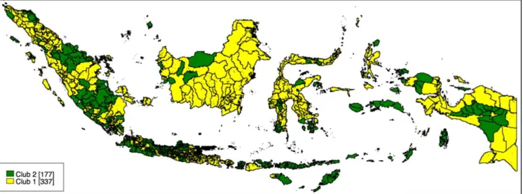
Geographical distribution of convergence clubs provide a few insights about regularities. Firstly, Figure 5 maps the distribution of GDP per capita convergence clubs. From the figure, the province effect seems significant since districts that belong to the same club tend to be in the same province (Barro, 1991; Quah, 1996). In other words, the clubs seem to be spatially concentrated. This result is consistent with the previous study’ result (Aginta et al., 2021). For example, the districts located in West Sumatera and the districts located in East Kalimantan tend to be gathered in Club 1.

Similarly, the districts located in Jambi and Centra Java tend to be gathered in Club 2.

This pattern applies to almost every districts.

In contrast with the previous study, this study does not identify any distinctive characteristics of the districts that belong to the clubs in terms of GDP per capita since the convergence is only broken down into two clubs—Club 1 for districts with relatively higher GDP per capita and Club 2 for districts with relatively lower GDP per capita. However, this study confirms one of the results of previous studies which outline the fact that districts which belong to the category of big cities or natural resource-rich regions, such as West Jakarta (part of the capital city), Kediri (largest tobacco producer), Morowali (recently developed nickel-based industrial area), Mamberamo Raya, Mimika, and Teluk Bintuni (natural resource-rich districts in the coastal area of Papua) are classified into higher income per capita convergence level.

Figure 5. Distribution of GDP per capita convergence clubs Source: Author’s calculation

Secondly, Figure 6 maps the distribution of household expenditure per capita convergence clubs. Similar to GDP per capita, the province effect appears to be significant, as districts located in the same province tend to congregate in similar clubs. Furthermore, the figure also shows a classic development gap between the west and east sides of Indonesia to a limited extent. In this case, most districts which belong to the fourth club are located in Papua, and two districts which belong to the fifth club are located in Papua and Southeast Sulawesi. However, it is important to notice that many districts located on the eastern sides of Indonesia are also grouped into Club 1 and

(19)

139

Club 2, which highlight a significant catching up effect in terms of household expenditure per capita.

Figure 6. Distribution of household expenditure per capita convergence clubs Source: Author’s calculation

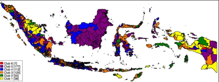
Thirdly, Figure 6 maps the poverty convergence clubs. Similarly, in terms of poverty rate, the province effect is still present as districts located in the same province tend to be grouped into similar clubs. In addition, the figure shows that districts that belong to Club 1 (the club of districts with highest poverty rate) are mainly concentrated in Papua and Riau, while the rest of the clubs are scattered all around Indonesia.

Figure 7. Distribution of poverty convergence clubs Source: Author’s calculation

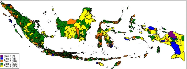
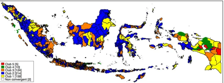
Finally, Figure 8 maps the distribution of convergence clubs in average years of schooling. Similar to other variable convergence clubs, the clubs of average years of schooling also tend to be spatially concentrated. Furthermore, the figure highlights a significant education gap between a few districts located in Papua and the rest of Indonesia, as the majority of districts that belong to Club 4 and all districts that belong to Club 5 are located in Papua.

(20)

140

Figure 8. Distribution of average years of schooling convergence clubs Source: Author’s calculation

CONCLUSION

In re-examining the regional inequality in Indonesia, this study goes beyond the previous literature by examining the convergence of a few other indicators namely household expenditure per capita, poverty and education besides GDP per capita using a method which is considered better than classical convergence methods. The results of this study suggest that regional GDP per capita, household expenditure per capita, poverty, and average years of schooling do not converge to the same single long-run equilibrium but are localized into a few convergence clubs. The evolution of disparities in terms of GDP per capita, household expenditure per capita, poverty, and average years of schooling is characterized by two, five, six, and five convergence clubs, respectively. The gap between the clubs with a higher level of convergence and the clubs with a lower level of convergence is significant and became wider during 2000–

2017. Furthermore, the analysis of regional disparities by the convergence clubs suggests the presence of spatial concentration among regions and a development gap between the east and west sides of Indonesia in terms of household expenditure per- capita, poverty, and average years of schooling. In this case, the districts with the lowest household expenditure per capita, the highest poverty rate, and the lowest average years of schooling are concentrated in the east parts of Indonesia.

From a policymaking point of view, this study suggests that policymakers should pay more attention to the convergence clubs' formation rather than focus on overall convergence. Furthermore, this study also emphasizes the fact that convergence in household expenditure, poverty, and average years of schooling should also become a focus of policymakers besides convergence in GDP per capita since they provide a detailed picture of inequality in household welfare, poverty, and education. Focusing on reducing inequality in terms of these different indicators across clubs is important in reducing the well-known overall disparities between West and East Indonesia.

Furthermore, because the majority of districts are spatially clustered, regional policy coordination at the provincial level would be more practical and effective in reducing regional inequality than centralized coordination.

(21)

141

ACKNOWLEDGEMENT

The author wishes to thank Prof. Budy P. Resosudarmo (The Australian National University) and Mrs. Diah Widyawati Ph.D. (Universitas Indonesia) for their input in the process of writing this article.

REFERENCES

Aginta, H., Gunawan, A., & Mendez, C. (2021). Regional income disparities and convergence clubs in Indonesia: new district-level evidence 2000-2017. Journal of the Asia Pacific Economy. DOI: 10.1080/13547860.2020.1868107

Barro, R. J. (1991). Economic growth in a cross section of countries. Quarterly Journal of Economics, 106(2),407–443. DOI: 10.2307/2937943

Barro, R., & Sala-i-Martin, X. (1992). Convergence. Journal of Political Economy 100 (2), 223-251. DOI: 10.1086/261816

Barro, R., & Sala-i-Martin, X. (2004). Economic Growth, MIT Press. Cambridge

Brodjonegoro, B. (2004). The effect of decentralization on business in Indonesia in Basri, M & van der Eng, P. Business in Indonesia: new challenges, old problem.

Singapore Institute of Southeast Asian Studies

Case, A., & Deaton, A. (2020). Deaths of despair and the future of capitalism.

Princeton University Press. Princeton

Corvers, F., & Mayhew K. (2021). Regional inequalities: causes and cures. OUP Public Health Emergency Collection 37(1),1-16. DOI:10.1093/oxrep/graa067

Du, K. (2017). Econometric convergence test and club clustering using Stata. The Stata Journal 17(4), 882– 900.

Floerkemeier, H., Spatafora, N., Venables, A., Cashin, P., & Cerra, V. (2021). Regional disparities, growth, and inclusiveness. IMF Working Paper vol. 2021(38).

International Monetary Fund. viewed 9 April 2022.

<https://www.elibrary.imf.org/configurable/content/journals$002f001$002f2021

$002f038$002farticle-A001

en.xml?t:ac=journals%24002f001%24002f2021%24002f038%24002farticle- A001-en.xml>

Garcia, J., & Soelistianingsih, L. (1998). Why do differences in provincial incomes persist in Indonesia? Bulletin of Indonesian Economic Studies 34 (1), 95-120.

DOI: 10.1080/00074919812331337290

Gunawan, A., Mendez, C., & Otsubo, S. (2021). Provincial income convergence clubs in Indonesia: identification and conditioning factors. Growth and Change: A Journal of Urban and Regional Policy 52(4), 2540-2575.

DOI:10.1111/grow.12553

Hill, H., Resosudarmo, B., & Vidyattama, Y. (2007). Indonesia’s changing economic geography. Bulletin of Indonesian Economic Studies 44(3), 407-435. DOI:

10.1080/00074910802395344

Holmes, C., & Mayhew, K. (2015). Over-qualification and skills mismatch in the graduate labour market. CIPD. viewed 10 April 2022.

<https://www.cipd.co.uk/Images/over-qualification-and-skills-mismatch- graduate-labour-market_tcm18-10231.pdf>

Kharisma, B., & Saleh, S. (2013). Convergence of income among provinces in Indonesia 1984-2008: a panel data approach. Journal of Indonesian Economy and Business 28(2), 167-187.

(22)

142

Kurniawan, H., De Groot, H., & Mulder, P. (2019). Are poor provinces catching-up the rich provinces in Indonesia? Regional Science Policy & Practice 11, 89–108.

DOI: 10.1111/rsp3.12160

Lessmann, C., & Seidel, A. (2017). Regional inequality, convergence, and its determinants- a view from outer space. European Economic Review 92, 110- 132. DOI: 10.1016/j.euroecorev.2016.11.009

Mendez, C. (2020). Convergence Clubs in Labor Productivity and its Proximate Sources. Springer

Mendez, C., & Kataoka, M. (2021). Disparities in regional productivity, capital accumulation, and efficiency across Indonesia: A club convergence approach.

Review of Development Economics 25(2), 790-809. DOI: 10.1111/rode.12726 Miranti, R. (2021). Is regional poverty converging across Indonesian districts? a

distribution dynamics and spatial econometric approach. Asia Pacific Journal of Regional Science 2021(5), 851-883. DOI: 10.1007/s41685-021-00199-3

Mishra, S. (2009). Economic inequality in Indonesia: trends, causes, and policy response. in Strategic Asia: Preparing for the Asian Century: 39-206, UNDP Nasution, A. (2016). Government decentralization program in Indonesia. ADB Working

Paper No. 601. Asian Development Bank, viewed 11 April 2022, <

https://www.adb.org/sites/default/files/publication/201116/adbi-wp601.pdf>

Phillips, P., & Sul, D. (2007). Transition modelling and econometric convergence tests.

Econometrica 75(6), 1153-1185. DOI: 10.1111/j.1468-0262.2007.00811.x Phillips, P., & Sul, D. (2009). Economic transition and growth. Journal of Applied

Econometrics 24(7),1771-1855. DOI: 10.1002/jae.1080

Quah, D. (1996). Empirics for economic growth and convergence. European Economic Review, 40(6), 1353–1375. DOI: 10.1016/0014-2921(95)00051-8

Rodriguez-Pose, A. (2018). The revenge of the places that don’t matter (and what to do about it). Cambridge Journal of Regions, Economy, and Society 11(1), 189-209.

DOI: 10.1093/cjres/rsx024

Santos-Marquez, F., Gunawan, A., Mendez, C. (2021). Regional income disparities, distributional convergence, and spatial effects: evidence from Indonesian regions 2010-2017. GeoJournal 2021, viewed 27 March 2022,

<https://link.springer.com/article/10.1007/s10708-021-10377-7>

Tirtosuharto, D. (2013). Regional inequality in Indonesia: did convergence occur following the 1997 financial crisis’ in Proceeding of the 23^rd Pacific Conference of Regional Science Association International (RSAI) and the 4^th Indonesian Regional Science Association (IRSA) Institute. Bandung

Vidyattama, Y. (2013). Regional convergence and the role of the neighbourhood effect in decentralized Indonesia. Bulletin of Indonesian Economic Studies 49(2),193- 211. DOI: 10.1080/00074918.2013.809841

(23)

143

Appendix 1: Robustness Check

Similar to Aginta et al. (2021) study which examines the convergence clubs at district level using imputed data, the robustness of data imputation in this article is checked by running the classical convergence (Beta & Sigma) tests using only 342 parent districts (the number of districts in 2000).

Table A1. Beta convergence

GDP Pc

Household Expenditure

Pc Poverty Average years of schooling α1 coefficient -0,019*** -0,012*** -0,044*** -0,002***