The regional variation of aboveground live biomass in old-growth Amazonian forests
Y A D V I N D E R M A L H I*w, D A N I E L W O O Dw, T I M O T H Y R . B A K E R § , J A M E S W R I G H T}, O L I V E R L . P H I L L I P S § , T H O M A S C O C H R A N Ek, P A T R I C K M E I Rw, J E R O M E C H AV E**, S A M U E L A L M E I D Aw w, L U Z M I L L A A R R O Y Ozz, N I R O H I G U C H I § § ,
T I M O T H Y J . K I L L E E N} }, S U S A N G . L A U R A N C Ekk, W I L L I A M F . L A U R A N C Ekk, S I M O N L . L E W I S § , A B E L M O N T E A G U D O***w w w, D AV I D A . N E I L Lzzz,
P E R C Y N U´ N˜ E Z VA R G A S § § § , N I G E L C . A . P I T M A N} } }, C A R L O S A L B E R T O Q U E S A D A § , R A FA E L S A L O M A˜ Ow w, J O S E´ N AT A L I N O M . S I LVAkkk****, A R M A N D O T O R R E S L E Z A M Aw w w w, J O H N T E R B O R G H} } }, R O D O L F O VA´ S Q U E Z M A R T I´ N E Zw w wa n d B A R B A R A V I N C E T Izzzz
*Oxford University Centre for the Environment, South Parks Road, Oxford, UK,wSchool of GeoSciences, University of Edinburgh, Darwin Building, Mayfield Road, Edinburgh, UK,§Earth and Biosphere Institute, Geography, University of Leeds, Leeds, UK, }Department of Geography, University of Southampton, Southampton, UK,kAgteca, Casilla Postal 6329, Santa Cruz, Bolivia,
**Laboratoire Evolution et Diversite´ Biologique, CNRS/UPS, Toulouse, France,wwMuseu Paraense Emilio Goeldi, Bele´m, Brazil, zzMuseo Noel Kempff Mercado, Santa Cruz, Bolivia,§§Instituto National de Pesquisas Amazoˆnicas, Manaus, Brazil,}}Center for Applied Biodiversity Science, Conservation International, Washington, DC, USA,kkSmithsonian Tropical Research Institute, Balboa, Panama, ***Herbario Vargas, Universidad Nacional San Antonio Abad del Cusco, Cusco, Peru,wwwProyecto Flora del Peru´, Jardin Botanico de Missouri, Oxapampa, Peru´,zzzFundacion Jatun Sacha, Quito, Ecuador,§§§Herbario Vargas, Universidad Nacional San Antonio Abad del Cusco, Cusco, Peru,}}}Center for Tropical Conservation, Duke University, Durham, NC, USA, kkkCIFOR, Tapajos, Brazil, ****EMBRAPA Amazonia Oriental, Bele´m, Brazil,wwwwINDEFOR, Facultad de Ciencias Forestales y Ambientale, Universidad de Los Andes, Me´rida, Venezuela,zzzzInternational Plant Genetic Resources Institute, Rome, Italy
Abstract
The biomass of tropical forests plays an important role in the global carbon cycle, both as a dynamic reservoir of carbon, and as a source of carbon dioxide to the atmosphere in areas undergoing deforestation. However, the absolute magnitude and environmental determi- nants of tropical forest biomass are still poorly understood. Here, we present a new synthesis and interpolation of the basal area and aboveground live biomass of old-growth lowland tropical forests across South America, based on data from 227 forest plots, many previously unpublished. Forest biomass was analyzed in terms of two uncorrelated factors:
basal area and mean wood density. Basal area is strongly affected by local landscape factors, but is relatively invariant at regional scale in moist tropical forests, and declines significantly at the dry periphery of the forest zone. Mean wood density is inversely correlated with forest dynamics, being lower in the dynamic forests of western Amazonia and high in the slow-growing forests of eastern Amazonia. The combination of these two factors results in biomass being highest in the moderately seasonal, slow growing forests of central Amazonia and the Guyanas (up to 350 Mg dry weight ha1) and declining to 200–
250 Mg dry weight ha1at the western, southern and eastern margins. Overall, we estimate the total aboveground live biomass of intact Amazonian rainforests (area 5.76106km2in 2000) to be 9323 Pg C, taking into account lianas and small trees. Including dead biomass and belowground biomass would increase this value by approximately 10% and 21%, respectively, but the spatial variation of these additional terms still needs to be quantified.
Keywords: Amazonia, biomass, carbon, soil fertility, tropical forests, wood density Received 10 January 2005; revised version received 18 August 2005; accepted 3 October 2005
Correspondence: Y. Malhi, Oxford University Centre for the Environment, South Parks Road, Oxford OX1 3QY, UK, tel: 144 (0)1865 285188, fax 144 (0)1865 271929, e-mail: [email protected]
r2006 The Authors
Introduction
The lowland tropical forests of South America account for about half of the world’s tropical forest area (FAO, 2001). They are estimated to account for 30% of global productivity (Royet al., 2001) and 25% of global biodi- versity (Groombridge & Jenkins, 2003). They are also being cleared at rapid rates (Achard et al., 2002), and are, thus, a major carbon source, equivalent to 5–10% of fossil fuel emissions in the 1990s (Achard et al., 2004).
Quantifying the amount of carbon stored and cycled in these forests is clearly important. In addition, there is accumulating evidence that old-growth tropical forests may be accelerating in growth (Lewis et al., 2004), recruitment and mortality (Phillips & Gentry, 1994;
Phillips et al., 2004), increasing in biomass (Malhi &
Grace, 2000; Bakeret al., 2004a) and shifting in ecologi- cal composition (Phillips et al., 2002; Laurance et al., 2004), but there is little understanding on the con- straints and determinants of current forest biomass.
The absolute magnitude and spatial variation of biomass in these forests are poorly quantified. Recent estimates of forest biomass have come from either interpolation of plot studies (Houghtonet al., 2001), or are based on a combination of modelling and remote- sensing approaches (Houghtonet al., 2001; Potteret al., 2001). Interpolation from site studies is hampered by the low number of systematically consistent compila- tions, or by only partial inventories of large trees or partial geographical coverage, such as RADAMBRASIL (Brown & Lugo, 1992; Fearnside, 1997). Model studies, on the other hand, are based on predictions of produc- tivity, and often incorporate untested assumptions about the relationship between gross photosynthesis, wood productivity and total biomass (Malhi et al., in preparation).
Here, we present a data synthesis and interpolation of results based on a compilation of biomass and basal area data across the South American lowland tropical forests. Many of these site data are previously unpub- lished, and/or are part of the RAINFOR network (Malhi et al., 2002) of Neotropical forest plots; other data are gathered from published or grey literature. We incorpo- rate data from 226 sites in eight South American coun- tries, to our knowledge the most spatially extensive dataset to date on neotropical forest biomass. We also include data from one well-studied central American site (Barro Colorado Island, Panama) in the analysis, but not in the spatial interpolations.
A novel feature that is accounted for in this analysis is biogeographic variation in mean forest wood density that is driven by shifts in tree species composition (Terborgh & Andresen, 1998). Analysing a subset of the plots presented here (Bakeret al., 2004b) found that
spatial variations in wood density play a major role in determining spatial variations in biomass. The mean wood density was found to be inversely correlated with wood productivity, with more dynamic forests having more light wood species. Moreover, aboveground wood productivity appears related to soil properties, but not to climate (Malhiet al., 2004). Our aim here is to assess how this variation in wood density affects regional patterns and total estimates of Amazonian forest bio- mass.
For the study here, we focus on South American tropical lowland forests. Ninety-five percent of these forests lie in a contiguous block in the Amazon and Orinoco basins and Guyana shield and are floristically interconnected; for convenient shorthand these will be referred to as ‘Amazonian forests’. The remaining 5% lie in small blocks west of the Andes, and in fragments in eastern Brazil and on the Atlantic coast. We focus solely on extrapolation of biomass from apparently undis- turbed old-growth forests. Hence, our extrapolated maps are estimates of the undisturbed biomass of Amazonian forests, and we do not try to account for human impacts such as forest degradation, cryptic forest impoverishment, which may be occurring at rates of 10–15 000 km2a1, and edge effects (Lauranceet al., 1997; Nepstad et al., 1999). Our aim is to understand how the background biomass of these forests varies with regional-scale environmental factors, not to quan- tify human impacts on these forests.
Materials and methods
Field sites, forest cover and climate
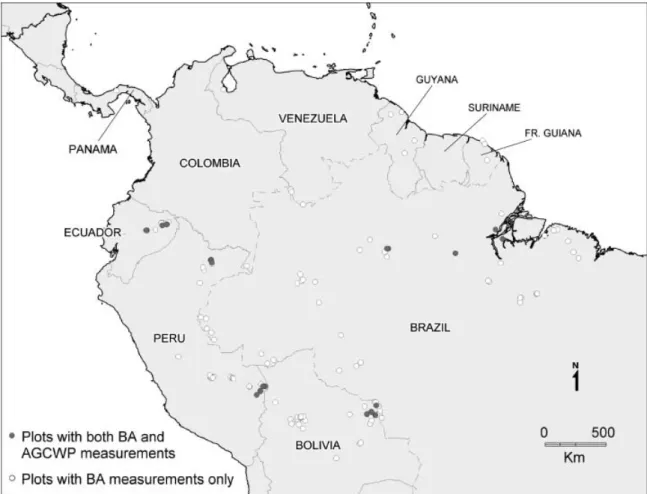
The data used in this study are listed in Table A1 in Appendix A, and mapped in Fig. 1. The dataset is a compilation of published values and unpublished data compiled by the authors within the RAINFOR project (Malhi et al., 2002, www.geog.leeds.ac.uk/projects/
rainfor), with the source indicated in Table 1. In total, there are 227 plots in the dataset, with reasonable distribution across Amazonia. The largest spatial gaps in our dataset are Colombia and the southern Brazilian Amazon. For the majority of sites (open circles in Fig. 1) only data on basal area were available (in general from published data). For a subset of sites (filled circles; bold type in the ‘biomass’ column in Table A1) the above- ground dry weight live biomass (henceforth ‘AGL biomass’) was directly estimated within the RAINFOR project, using individual tree diameter data and taxon- omy to directly account for wood density and the size-class distribution of stems (Baker et al., 2004b).
Only trees with diameter at 1.3 m (dbh)410 cm were 2 Y. M A L H I et al.
r2006 The Authors
Fig. 1 Forest site locations where basal area measurements have been taken in lowland South American tropical forests. Filled circles indicate sites where the availability of taxonomic data permitted direct calculation of mean wood density; open circles indicate sites where only information on total basal area was available.
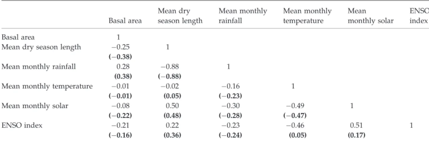
Table 1 Cross-correlation matrix of forest plot basal area against various climatic variables, including the multi-variate ENSO index
Basal area
Mean dry season length
Mean monthly rainfall
Mean monthly temperature
Mean monthly solar
ENSO index
Basal area 1
Mean dry season length 0.25 1
(0.38)
Mean monthly rainfall 0.28 0.88 1
(0.38) (0.88)
Mean monthly temperature 0.01 0.02 0.16 1
(0.01) (0.05) (0.23)
Mean monthly solar 0.08 0.50 0.30 0.49 1
(0.22) (0.48) (0.28) (0.47)
ENSO index 0.21 0.22 0.23 0.46 0.51 1
(0.16) (0.36) (0.24) (0.05) (0.17)
Figures in normal type are for all forest plot data; figures in bold type in brackets are after removal of 28 outlier plots as described in the text.
ENSO, El Nino-southern oscillation.
r2006 The Authors
considered in plot-level estimates of biomass; small trees and lianas may account for up to a further 10%
of biomass (Phillipset al., 1998; DeWalt & Chave, 2004).
Biomass for these plots was estimated using individual tree allometric relationships derived from direct sam- pling in central Amazonia, with additional incorpora- tion of wood density data for each species; details are given in Bakeret al. (2004b).
The approach to estimate biomass applied here tries to take into account spatial variation in basal area, stem size distribution and wood density. One factor that is still not accounted for is spatial variation in allometry (i.e. the tree height and biomass supported for a given tree basal area). The data that exist to date (T. Baker, unpublished data) give no indication of a clear relation- ship between allometry and environmental factors, although it would be expected from hydrological con- siderations (Meinzer et al., 1999; 2001) that tree height per unit basal area would reduce with increasing dry season length. As the biomass estimates derived here apply an allometric relationship derived for the central Amazon near Manaus, it is likely that tree height and biomass at the dry margins of Amazonia will be over- estimated.
We concentrate our analyses and extrapolations on the continuous lowland tropical rainforest region centred on the Amazon Basin. The dry limits of ‘rain- forests’ are rather arbitrary and vary according to source and climatic dataset applied. Here, we use a definition of a lowland tropical rainforest as equivalent to the ‘rainforest’ plus ‘tropical moist forest’ categories in the FAO Global Forest Resources Assessment 2000 (FAO Forestry Paper 140, data available online at http://www.fao.org/forestry/fo/fra), and at an eleva- tion less than 1000 m. The FAO defines tropical forests as forests with mean temperature in all months over 181C, with 0–3 dry months (rainforests) or 3–5 dry months (moist deciduous forest), where dry months are defined as months where total precipitation in millimeters is equal to or less than twice the mean temperature in degree Celsius.1 Some estimates of tropical forest area also include the ‘tropical dry forest category’. However, this category frequently grades into woody savanna regions, and is excluded from the current analysis. The forest cover map was
coarsened to 0.51 resolution to be compatible with the climate dataset. Our study area included significant areas outside the Amazon watershed, in particular large areas of the Orinoco Basin, the Guyana lowlands and the Brazilian periphery east of the mouth of the Ama- zon. However, these areas form a phytogeographic continuum with Amazon lowland rainforest, and hence, it is reasonable to adopt the shorthand ‘Amazo- nia’ to describe this entire lowland tropical forest region. Other recent maps of forest cover (Achard et al., 2002; DeFrieset al., 2002; Eva et al., 2004) differ at the margins from the FAO map; hence estimates of the total biomass of Amazonian rainforests will also depend on the spatial extent of forests in different analyses. This topic is not addressed here. For the definition used here, the total extent of Amazonian forests is 5.76106km2.
The climatic and soils variations across the region were discussed by (Malhiet al., 2004). In summary:
(i) There is a general trend of increasing rainfall and decreasing seasonality heading towards north- western Amazonia, but also high rainfall on the eastern Brazilian and Guyanese coasts;
(ii) The El Nino-Southern Oscillation (ENSO) has great- est influence in northern Amazonia, and in particu- lar often leads to episodic droughts in central and eastern Amazonia. ENSO has little consistent influ- ence on rainfall in southwestern Amazonia.
(iii) Sunshine is higher but more seasonal at the north- ern and southern margins of Amazonia, where the climate shifts towards ‘outer tropical’ and there are long dry seasons.
(iv) The lowland Amazonian plain consists of low plateaux dissected by river values, and rises very gradually in mean elevation from sea level in the east to 2–300 m a.s.l. in the west. The Brazilian and Guyanese crystalline shield rise to the north and south, with typical elevations of 600–1000 m, and the Andes mountain chain bounds Amazonia to the west.
(v) The most highly weathered soils generally occur in the eastern Amazonian lowlands (Sombroek, 2000), intermediate fertilities are generally found on the crystalline shield regions, and highest fertilities in the Andean foothills, and on sediment-rich flood- plains throughout the region. We employ the Co- chrane map of soils (www.agteca.com) as our basic soil map. This map does not cover the Guyanas and some sections of eastern Amazonia; for these regions we employed the FAO world soils map.
The reclassification of these soil maps into eight basic soil categories is described in a companion paper (Malhiet al., in preparation).
1Some of the sites presented in Table A1 are estimated to have dry seasons greater than 5 months. This arises from a mismatch between the climatology used for the original FAO map and the climatology we use here – both climatologies are based on sparse data sets and subject to uncertainty in local details. For simplicity where retain the use of the two data sets despite the contradictions at the forest margins.
4 Y. M A L H I et al.
r2006 The Authors
Analysis methodology
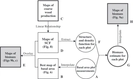
Our approach here, is as follows (letters refer to the flow diagram in Fig. 2):
(1) interpolate the available plot data on basal area per hectare (A) to generate maps of the variation of basal area across South American tropical forests (B);
(2) examine the relationship between biomass, basal area and coarse wood productivity for a subset of plots where these parameters were directly esti- mated by Bakeret al. (2004b) and Malhiet al. (2004);
(3) apply the relationship derived in (2) to two different maps of wood productivity derived by Malhiet al.
(in preparation) to produce maps of the structural conversion factor required to convert a basal area measurement to a biomass estimate (D);
(4) directly overlay the map of basal area (B) with the map of the conversion factor (D) to produce a map of biomass (E);
(5) as an alternative approach, use the map of conver- sion factor (D) to extract the conversion factor for each plot where only basal area information is available (F), and thus, derive an estimate of bio- mass for each plot (G) and interpolate these to arrive at alternative maps of biomass (H).
Spatial interpolation of the plot data was investigated using three different approaches: kriging, spline inter- polation and inverse distance weighting (IDW). Kriging and spline interpolation approaches performed poorly because the high variability of biomass between plots at local scales. Basal area shows considerable local and landscape scale variability (in contrast to productivity,
for example, which is dominated by regional-scale variation: Malhi et al., 2004). Consequently, the least sophisticated interpolation method (IDW) was found to be most appropriate, and was applied using the geos- tatistical analysis tool in ArcMAP (ESRI, Redlands, CA, USA). For any value of a continuous variable B(x,y) interpolated between theNneighbouring points (xi,yi) in the search window(i51, 2, . . .N), the IDW interpola- tion at point (x,y) is
Bðx;yÞ ¼ PN
i¼1wi:Bðxi;yiÞ PN
i¼1wi
;
where
wi¼hðxxiÞ2þðyyiÞ2ip=2
:
The power, p, is an adjustable parameter that controls the rate of decline of the weighting function. For our purposes the most appropriate setting was p51: this resulted in a smoothed interpolation with a large num- ber of neighbouring points having some influence, with only a slow decline in weighting function with distance.
Results
Spatial interpolation of basal area
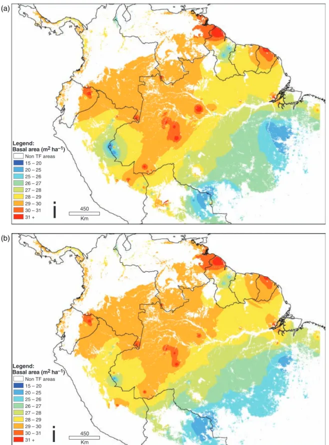
Our first step is to use the plot measurements of basal area (A in Fig. 2) to produce a best estimate map of basal area (B in Fig. 2). An IDW interpolation of all basal area measurements is shown in Fig. 3a. A feature that stands out is local ‘bulls-eyes’ driven by individual plots with unusually high or low values. This contrasts with
Maps of coarse
wood production
Maps of SCF (Fig. 8)
Best map of basal area
(Fig. 6)
Basal area plot measurements Structure and density function for each plot
Biomass estimate for
each plot Maps of biomass (Fig. 9a)
Maps of biomass (Figs 9b, c)
Overlay
Extract
Interpolate
Interpolate
Linear Relationship
A E
D C
B
H
F
G
Fig. 2 A flow diagram indicating the analysis pathways presented in this paper. Squares indicate maps, circles indicates table of values for each plot, shaded squares indicate the end-products: maps of biomass. Details of the analysis pathways are presented in the text.
r2006 The Authors
Legend:
Basal area (m2 ha–1) Non TF areas 15 – 20 20 – 25 25 – 26 26 – 27 27 – 28 28 – 29 29 – 30 30 – 31 31 +
Legend:
Basal area (m2 ha–1) Non TF areas 15 – 20 20 – 25 25 – 26 26 – 27 27 – 28 28 – 29 29 – 30 30 – 31 31 +
i
450Kmi
450Km(a)
(b)
Fig. 3 (a) A simple interpolation of 227 basal area measurements using inverse distance weighting across lowland South American tropical forests; (b) an interpolation of 199 basal area measurements (28 plots have been removed as ‘outliers’ – details given in the text).
6 Y. M A L H I et al.
r2006 The Authors
maps of forest productivity, which are much smoother.
This feature arises because basal area is much more affected by local landscape features (e.g. local topogra- phy, or recent natural disturbance) and such local variations can swamp regional patterns. In addition, 1 ha sample plots may not be large enough to accurately sample the variance in biomass introduced by large trees (Chave et al., 2003), but may be sufficient for assessment of wood productivity, as evidenced by the greater similarity in wood productivity values between neighbouring plots (Malhiet al., 2004).
As our interest here is to examine broad regional patterns, we employed a filter to remove locally anom- alous plots and smooth the data set. The approach identified clusters of forest plots (of varying sizes) and local anomalous plots were removed if the value for the plot fell outside the range (mean value of neigh- boursstandard deviation of neighbouring values threshold), where the threshold was varied between values of 1.0 and 1.8.
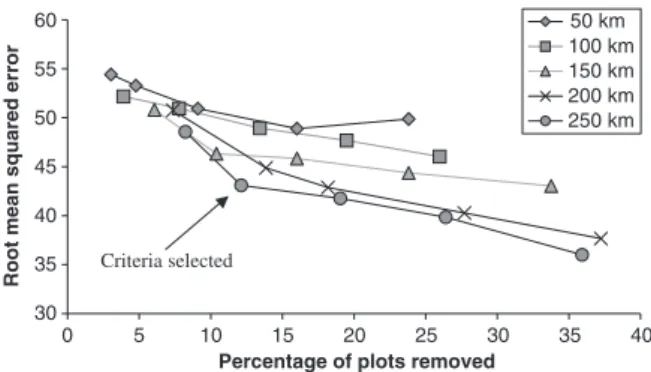
The effect of removing anomalous plots is shown in Fig. 4. Removing outliers improves the predictive power of the interpolation (as would be expected), but with greater data removal there is greater danger of losing genuine regional variation. We adopted a com- promise approach of using a search radius of 250 km and a threshold value of 1.6 for anomaly removal. This corresponds to an inflection in Fig. 4 which indicates an optimal compromise between a significant improve- ment in predictive power and minimum data shedding.
This removes 28 plots (12% of plots; removed plots are indicated with an asterisk in Table A1), and improves the cross-validation statistics by 22%. The interpolated may of basal area with outliers removed is shown in Fig. 3b. The ‘bulls-eye’ pattern has reduced in intensity, although not disappeared completely.
The relationship between basal area and climatic variables was explored by cross-correlation analysis (Table 1). The cross-correlations were significantly im- proved by the removal of locally anomalous plots. The strongest correlation (0.38) was found to be with dry season length and/or total annual rainfall (these two climatic variables were strongly correlated), and this relationship was explored further.
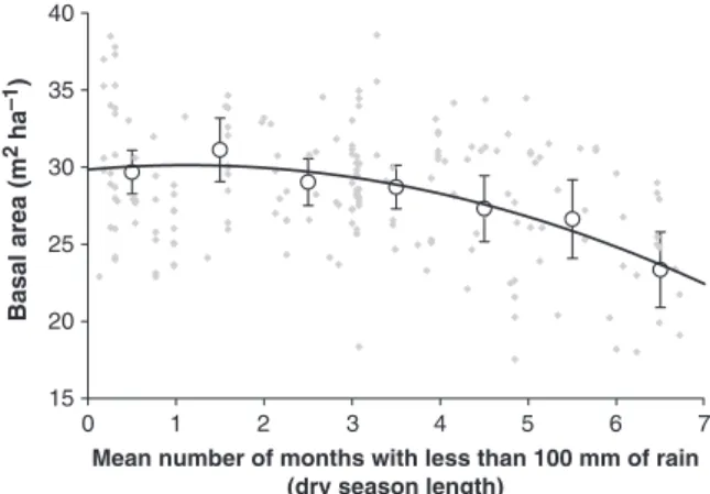
Figure 5 plots the basal area against dry season length. There is substantial site-to-site variability, indi- cating that local landscape controls dominate over regional trends. There is little evidence of any relation- ship for moderate seasonality (less than 4 months dry season), but evidence of a general decline in the basal area of tropical forests with increasing water stress for longer dry season lengths. This is to be expected as root competition for dry season water resources intensifies, and the ground surface is able to support
less stem water uptake per unit area (e.g. Meinzeret al., 1999).
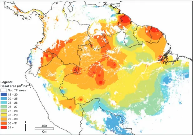
A revised interpolation of basal area with dry season length factored in (Fig. 6) was conducted by calculation of a smooth mean basal area field from the basal area–
dry season length relationship in Fig. 5, and then IDW interpolation and superposition of the residuals of each data point relative to this mean field. There was no significant correlation between the residuals and any other climatic variable. The major difference from Fig. 3
30 35 40 45 50 55 60
0 5 10 15 20 25 30 35 40
Percentage of plots removed
Root mean squared error
50 km 100 km 150 km 200 km 250 km
Criteria selected
Fig. 4 The root mean squared error value obtained by cross validation of inverse distance weighting interpolations of basal area, plotted against the percentage of local anomalous plots removed using different thresholds for outlier identification. The different lines represent different sized search radii employed by the outlier identification algorithm. The arrow indicated the selected optimum outlier removal procedure (threshold51.6, search radius5250 km), a compromise between maximizing error reduction and minimizing data shedding.
15 20 25 30 35 40
0 1 2 3 4 5 6 7
Mean number of months with less than 100 mm of rain (dry season length)
Basal area (m2 ha–1)
Fig. 5 Plot measurements of basal area (with 28 local outlier plots removed) plotted against dry season length. Grey dia- monds indicate individual plot data, open circles are binned means, error bars are 95% confidence limits. The polynomial trend line is fitted through the binned means: y50.22x21 0.50x129.84 (r250.93). A polynomial fit through individual points is almost identical: y50.29x211.00x128.87 (r250.18).
r2006 The Authors
is in south-eastern Amazonia, where there is a paucity of field plots. This extra information gained from in- corporating dry season length into the model suggests that the wetter forests extend further into this region than suggested by direct spatial interpolation of plot data, and hence, basal area in this region is higher than expected. Another feature is a reduction of predicted basal area in the dry region in the central Guyanas, which is consistent with the available plot data in the region. We consider this interpolation to be our current best estimate of the spatial variation of basal area in Amazonia.
Structural and density factor
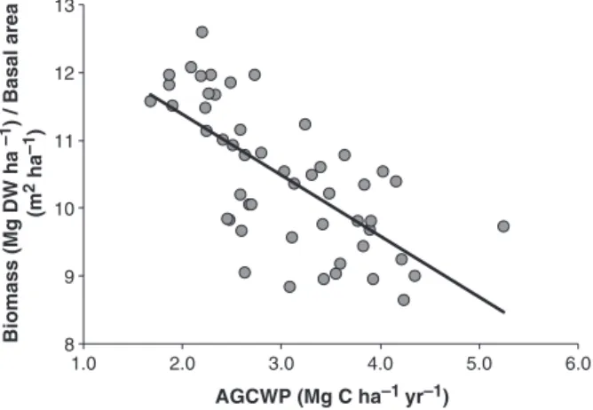
Our next step is to relate basal area to biomass. We will refer to the ratio between aboveground live biomass (of trees410 cm dbh) and basal area (i.e. the mean amount of biomass supported per unit of forest basal area) as the structural conversion factor (SCF). Baker et al., (2004b) found that variations in wood density and size class distribution have a significant influence on the SCF, and that spatial variations in SCF appeared more important than variations in basal area in determining the spatial pattern in aboveground biomass. Figure 7
demonstrates that the SCF is related to wood produc- tivity, with more productive forests having lower wood density. There is, however, some variance that is not
Legend:
Basal area (m2 ha–1) Non TF areas 15 – 20 20 – 25 25 – 26 26 – 27 27 – 28 28 – 29 29 – 30 30 – 31
31 +
i
450KmFig. 6 An interpolation of forest basal area across lowland South American tropical forests incorporating the relationship with dry season length described in Fig. 5 (with 28 local outlier plots removed).
8 9 10 11 12 13
1.0 2.0 3.0 4.0 5.0 6.0
AGCWP (Mg C ha–1 yr–1) Biomass (Mg DW ha –1) / Basal area (m2 ha–1)
Fig. 7 The relationship between the structural conversion fac- tor, SCF (5plot aboveground live biomass/plot basal area) and aboveground coarse wood productivity for 56 lowland Amazo- nian forests. Biomass and basal area values are derived from Bakeret al. (2004), productivity values from Malhiet al. (2004).
The least-squares linear fit (black solid line) is y50.90x113.19, r250.48.
8 Y. M A L H I et al.
r2006 The Authors
related to wood density, and is instead influenced by size-class distribution.
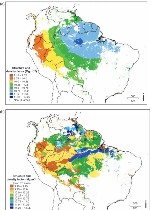
Using the relationship shown in Fig. 7, we mapped the spatial variation in the SCF (D in Fig. 2) using the maps of wood productivity generated in Malhiet al. (in preparation; C in Fig. 2). Two productivity maps were used: one that was a direct kriging interpolation of the productivity data, and a second based on a ‘painting- by-numbers’ approach (Schimel & Potter, 1995) that assumed productivity was related to soil type (both maps are shown in Fig. 8). Details of the extrapolation of productivity data will be given in Malhi et al. (in preparation). The SCF varies by about 30%, between 9 and 12 Mg DW m2basal area. Both maps show a simi- lar broad regional pattern with lower SCF being found in the more dynamic western Amazonian forests, and high values in north-east Amazonia. The two maps differ in smoothness and in detail. If the spatial varia- bility is predominantly driven by soil prperties (Malhi et al., 2004), the map suggests that the highest values of SCF are found in the old, highly weathered oxisols along the main Amazon valley, and intermediate values are to be found on the crystalline shield to the north and south. The soils-based map gives spatial details but the consistency of the SCF : soil relationship and the local details of the soils map are still uncertain, so these local details should be treated as tentative. The calculations in the rest of this paper will be based in parallel on both the kriging and soils-based interpolations. The basal area and SCF show almost no spatial correlation and can be treated as independent influencing factors on biomass (the correlation coefficient between plot values of basal area and kriging-derived SCF was 0.02; between basal area and soils map-derived SCF it was0.05).
Maps of biomass
Having derived maps of basal area (B in Fig. 2) and SCF (D in Fig. 2), our next step was to estimate the SCF and biomass for each plot (F and G in Fig. 2). Where plot biomass had been directly derived from the individual tree data using a consistent protocol as described by Baker et al. (2004b), this value was preferred. Where such directly calculated biomass was not available, we extracted an estimate of SCF for each plot from the maps in Fig. 8, and multiplied this by the reported basal area to calculate the plot biomass. These values are listed in Table A1.
We then employed three approaches to produce region-wide maps of biomass:
1. Use the allometric relationship derived for the central Amazon with no allowance for spatial variation in SCF.
2. Directly overlay the maps of basal area (B in Fig. 2) and the maps of the SCF (with one map each for the kriged and soil-based interpolations; D in Fig. 2) to produce a map of biomass (E in Fig. 2).
3. Directly interpolate the derived biomass values for each site (G in Fig. 2) to produce an alternative map of biomass (H in Fig. 2). We used the same procedure and thresholds to remove local anomalies as outlined for the basal area interpolation above.
The resulting maps of biomass are shown in Fig. 9.
There are significant differences in details between the kriging-based and soils-based maps, but the overall patterns are similar. The two different routes to calcu- lating biomass (E and H in Fig. 2) yield very similar results, with the exception that H does not factor in the relationship between basal area and dry season length.
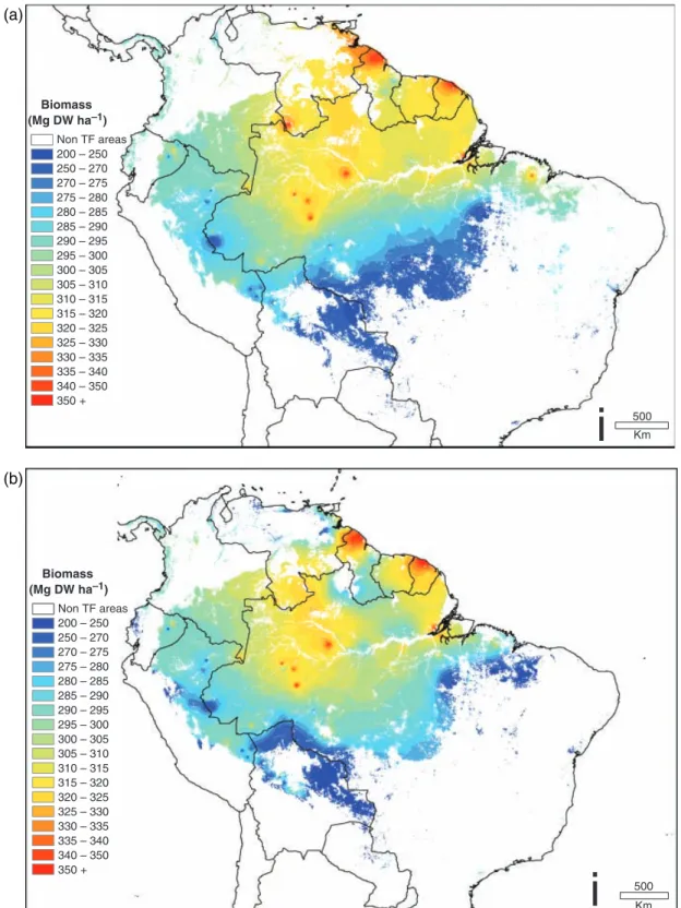
Hence, we consider Fig. 9b and c to be our best estimates of forest biomass. In general, biomass is calculated to be highest in central Amazonia and on the Guyana coast. This represents an optimum combi- nation of high basal area (related to short dry season length) and high wood density (related to low produc- tivity and probably to infertile soils). As we head to aseasonal northwestern Amazonia, basal area increases but is offset by the increasing abundance of low wood density species. Heading towards the dry southern and northern margins, wood density is moderately high, but basal area drops off because of limited water availabil- ity. The coastal areas of Brazil and the Guyanas also appear to have high biomass, a combination of the high basal area sustained by oceanic front rainfall, and high wood density on infertile soils. Comparing the soils- based map (9c) with the kriging map (9b), the soils map suggests that the high wood density zone may extend further northwest into the infertile soils of lowland Colombia and Venezuela, and snake east along the lowland corridor bordering the Amazon river, but the broad patterns are similar. Overall, regional mean bio- mass over the forest area of 5.76106km2 varies be- tween 250 and 350 Mg DW ha1yr1. The mean value reported by Baker et al. (2004b) was 298 (51) Mg DW ha1, suggesting that the core dataset used by Bakeret al. (2004b) was well distributed.
The per hectare and total carbon stocks (over area 5.76106km2) for the lowland Amazonian forests cal- culated by the different approaches are tabulated in Table 2. The most apparent feature is that incorporation of spatial variability in the SCF reduces the estimated total carbon stocks by about 8% from 92 to 83–86 Pg C (top row vs. bottom two rows). This is because the default allometric relationships used are based on studies in the central Amazon near Manaus, a region shown in Fig. 9 to have among the highest biomass r2006 The Authors
Structure and density factor (Mg m–2)
Structure and density factor (Mg m–2)
9.15 – 9.75 9.75 – 10.0 10.0 – 10.25 10.25 – 10.5 10.5 – 10.75 10.75 – 11.0 11.0 – 11.25 11.25 – 12.25
9.15 – 9.75 9.75 – 10.0 10.0 – 10.25 10.25 – 10.5 10.5 – 10.75 10.75 – 11.0 11.0 – 11.25 11.25 – 12.25 Non TF areas
Non TF areas
500
Km
i
500
Km
i
(a)
(b)
Fig. 8 Interpolation of the structural conversion factor across lowland South American tropical forests derived using the linear relationship presented in Fig. 7 with (a) a map of aboveground coarse wood productivity (AGCWP) interpolated by ordinary kriging, and (b) a map of AGCWP based on soil categories.
10 Y . M A L H I et al.
r2006 The Authors
Biomass (Mg DW ha–1)
Non TF areas 200 – 250 250 – 270 270 – 275 275 – 280 280 – 285 285 – 290 290 – 295 295 – 300 300 – 305 305 – 310 310 – 315 315 – 320 320 – 325 325 – 330 330 – 335 335 – 340 340 – 350 350 +
Biomass (Mg DW ha–1)
Non TF areas 200 – 250 250 – 270 270 – 275 275 – 280 280 – 285 285 – 290 290 – 295 295 – 300 300 – 305 305 – 310 310 – 315 315 – 320 320 – 325 325 – 330 330 – 335 335 – 340 340 – 350 350 +
500
i
Km500
i
Km(a)
(b)
Fig. 9 Interpolations of biomass of lowland South American tropical forests: (a) calculated by interpolating biomass estimates generated at each plot (with 25 local anomalous plots removed using a search radius of 250 km) using inverse distance weighting (5Box H in Fig. 2); (b) calculated by overlaying the best basal area estimate (Fig. 6) with maps of the structure and wood density function (Fig. 8), using kriged interpolations for both maps (5Box E in Fig. 2); (c) as for (b) but using soils-based interpolations instead of kriged interpolations.
r2006 The Authors
values in Amazonia. The particular method of spatial interpolation used has little effect on estimates of total biomass: the soils-based interpolations (bottom row) tend to give a value 2–3% lower because they suggest that poorly sampled regions of the Amazonian crystal- line shield may have high fertility and lower wood density than simple kriging of the existing plot data would suggest.
The values cited here are for aboveground woody biomass of all live trees410 cm dbh. To arrive at total biomass carbon stocks we need to include a number of extra terms, such as the biomass of trees o10 cm dbh, the biomass of lianas, dead biomass, and belowground carbon. These extra terms have been estimated for some forest plot sites, but as their spatial variation is unclear we do not attempt to map their spatial variability, but rather include mean values as multiplicative factors to arrive at estimates of total biomass carbon stocks. To be consistent with Phillips et al. (1998), we estimate the biomass of trees lesso10 cm to be an additional 6.2%, based on forest plots in the Manaus region, and the biomass of lianas to be 3.7% of total aboveground tree biomass, based on several plots in western Amazonia.
Dead wood biomass has been estimated at a number of sites and ranges between 6.41.6 Mg C ha1over 10 ha in southern Peru (Baker et al., submitted) and 25–
30 Mg C ha1at two sites in eastern Amazonia (Keller et al., 2004; Riceet al., 2004), and Houghtonet al. (2001) report a mean value of 10% of live biomass, the value that is applied here. Belowground biomass has been measured at only a few sites, and Houghtonet al. (2001) report a mean value of 21% (range 13–26%) of above- ground live tree biomass; that value is applied here.
Applying these approximate multiplicative factors uni- formly to our previous estimate of aboveground live woody biomass (83–86 Pg C), we estimate that the total aboveground live woody biomass is about 91–95 Pg C, the total aboveground woody biomass is about 100–
104 Pg C, and the total woody biomass is 121–126 Pg C.
Discussion
Using data from 227 forest plots, we have explored the spatial variation of aboveground live biomass in Ama- zonia, with particular emphasis on accounting for var- iations in basal area and wood density. Although there is substantial site-to-site variability, we were able to determine the somewhat opposing trends in these two factors, both of which are important determinants of AGLB. Wood density tends to peak in the slow growing forests on infertile soils in eastern lowland Amazonia and the Guyanas, and is lowest in the much more dynamic forests of western Amazonia. Basal area gen- erally declines with increasing dry season length, for
regions with a 4 months or longer dry season. The superposition of these two factors indicates that bio- mass is highest in central Amazonia and the Guyanas, and is about 15% lower in the more dynamic west, and lowest in the dry fringes to the south and north.
The estimates of aboveground live biomass were based on two parameters: basal area and structural conversion factor. These two parameters seem fairly independent at regional scales – basal area is related to hydraulic considerations and hence to dry season length, whereas the structural conversion factor is re- lated to productivity and hence probably to soil fertility (Malhiet al., 2004). The combination of these two factors leads to maximum biomass is wet regions with low wood productivities and infertile soils, such as central Amazonia and the Guyana coast, and lower biomass in dynamic western Amazonia, and the dry southern and northern fringes.
A number of the removed ‘anomalous plots’ show evidently unusual properties (e.g. the liana-dominated forests at CHO-1 CHO-2, XIN-01 and XIN-02, the bamboo-dominated forests RES-06 and CAM-02, fire- affected forest at NKT-01 and NKT-02, the gallery forests NKE-02, NKG-01). While these obviously influ- ence regional analyses of biomass, it is not surprising that the ecological and/or historical factors that cause their unusual properties are not captured in this broad analysis. Other forest plots are suspected of being subject to a majestic forest sampling bias where the original investigators deliberately selected high bio- mass stands (e.g. BEN-5, BEN-10, BEN-9: ‘contains one of the last remaining stands ofSwietenia macrophylla in the reserve reaching seven trees per hectare’). Others may be recently affected by a local natural disturbance (BDF-04 suffered recent high mortality from a La Nin˜a- related flooding event). A number of the anomalous sites have no obvious explanation, which may reflect the random influence of a single very large tree within the sample plot, or our ignorance of detailed sampling methodologies, or else additional factors that are not considered in this analysis.
Uncertainties
Tree height allometry.Probably the most important factor that has not been included here is spatial variability in height allometry, which would be expected to show a similar pattern to basal area and decrease with increasing dry season length as hydraulic constraints on tree height become more severe. Hence, biomass would drop off more rapidly at the dry extremes.
However, it is not clear whether height allometry shows any variation under moderate dry season conditions, and hence, whether the central Amazonian 12 Y . M A L H I et al.
r2006 The Authors
peak in biomass would be shifted towards more aseasonal regions.
The relationship between wood density and allometry. In adopting the approach of Baker et al. (2004b), we are assuming that allometries can be scaled linearly by wood density. It is plausible that low wood density trees have different architecture than high wood density trees. However, in their comprehensive assessment of tree allometry of 2410 trees, Chave et al. (2005) found that their null hypothesis of a linear relationship between wood density and aboveground biomass was not rejected, suggesting there is little evidence of a nonlinear scaling by wood density. Moreover, Chave et al. (2005) found no significant difference in allo- metries from South American and South-East Asian forests (constructed by lumping all species), despite the fact that these forests share almost no common genera, and very different dominant families. This again suggests no significant allometric differences between major tree dicot families.
Biased land-form selection.There may be some biases in site selection in our plot network (e.g. plateaux are favoured over steep slopes, accessible flood plains are favoured over ‘interior’ forests). In the soils-based interpolation, we try to account for landform using by including the various ‘facets’ in the Cochrane and FAO maps (e.g. if the map described a land form as 90%
plateau, 10% river valley, these are assigned different values). Given that there is little difference between the soils-based and kriging interpolations intotal biomass, it is unlikely that our estimate in total biomass will be strongly affected by this bias, although the details of regional patterns may vary. A remote sensing analysis to evaluate the landscape context of a number of the RAINFOR plots is currently under way.
Biased sampling of disturbance-recovery dynamics. Old growth tropical forests have a natural disturbance- recovery dynamic (e.g. sites are hit by occasional large tree falls/blowdowns, followed by slow recovery in biomass until the next infrequent disturbance). In setting up forest plots, it is possible that sites that recently underwent strong natural disturbance (e.g.
storm blowdowns) were avoided. The would lead to an overestimate of the background biomass of old- growth forest biomass. The magnitude of such a bias is likely to be small, but is difficult to quantify and requires detailed exploration of the disturbance- recovery dynamics of Amazonian forests.
The effect of wrinkled topography.Most of the forest plots are established in terms of a fixed ground area. In
regions of significant slopes or undulating topography, the biomass per unit area of the Earth’s surface could be significantly higher. This ‘wrinkled topography’ effect would increase biomass estimates in geomorphological transition zones such as the periphery of the Andes, and the Brazilian and Guyanan shields. It should be straightforward to estimate this effect with high- resolution digital elevation data.
Quantification of uncertainty in region-wide totals The above sources of uncertainties in our biomass totals can be classified into two categories (Chaveet al., 2004):
sampling uncertainties caused by partial sampling of a landscape that is heterogeneous at many scales, and systematic biases caused by errors in methodology of biomass measurement or analysis, such as incorrect allometric equations. Stochastic sampling uncertainties in our estimates of biomass are likely to be smaller when considering basin-wide totals, as opposed to accurate prediction of biomass at specific sites. Table 2 gives us some insight into the likely sensitivity of basin- wide totals to sampling uncertainties:
(i) The total area of forest sampled (excluding the 50 ha Panama site) is 366.1 ha, which can be di- vided into approximately seven regions of 50 ha each. The standard error of mean basal area over the entire dataset is about 1% (over each region it is about 4%). With a normal distribution, the 95%
confidence limits would be 2% and 8%, respec- tively. This is consistent with the findings of Keller et al. (2001) and Chave et al. (2003), who reported that approximately ten 1 ha plots are required to bring 95% confidence limits within 20%, and 26 ha to bring these limits within 10%. Assuming well- distributed sampling, the random sampling uncer- tainty in basin-wide and regional basal area esti- mates would be 2% and 8%, respectively (95%
confidence).
(ii) Uncertainty in the use of allometric models con- tributes a systematic uncertainty of about 13%
(Chaveet al., 2005).
(iii) Imposition of the SCF reduces estimates of total regional biomass by 7%; the variation in assump- tion about the exact distribution of SCF causes a systematic bias of about 3% in final biomass (rows in Table 2b).
(iv) Similarly, removal of outliers, and comparison with the mean of the sample plots has only modest influence on basin-wide totals, of order 3% (col- umns in Table 3b). This suggests that the spatial sampling bias contributes an uncertainty less than 5% in basin-wide totals.
r2006 The Authors
(v) Other uncertainties listed above are currently more difficult to quantify, but in total they are unlikely to exceed 10%.
If all these uncertainties were strongly correlated, the total uncertainty in biomass estimates would be about 35%, if they were independent the total uncertainty would be 18%. Hence, 25% is a conservative estimate of uncertainty in basin-wide biomass totals, with sys- tematic uncertainty in allometric relationships being the biggest contributing factor. Applying an uncertainty of 25% to our previous calculations, we estimate that the total aboveground live woody biomass is 93 23 Pg C, the total aboveground woody biomass is about 10226 Pg C, and the total woody biomass is 123 31 Pg C.
Comparison with previous estimates for Brazilian Amazonia
How does our estimate of the spatial patterns and total biomass of Amazonian forests compare with previous estimates? Houghtonet al. (2001) compared a variety of
maps of biomass for the Brazilian Amazon only. From our study mean biomass values were extracted from Fig. 9 for forested regions of the Brazilian Amazon only (area 3.60106km2 compared with total Amazonian forest area 5.76106km2), and these are presented in Table 3 for comparison with various values reported by (Houghtonet al. (2001). For compatibility, the 30% cor- rection that Houghtonet al. applied for dead wood and below-ground biomass has been removed, (i.e. we are considering aboveground live biomass only). A 10.1%
correction for trees o10 cm dbh and lianas has been retained for our analysis to be compatible with Phillips et al.(1998). For the field measurements summarized by Houghtonet al. (2001), it was not clear which data sets included small trees and lianas, and which did not.
Allowing for regional variations in basal area and SCF, we calculate the mean AGL biomass of Brazil Amazonian moist forests to be about 160 Mg C ha1 (6–10% lower than if a central Amazonian struc- ture factor had been uniformly applied), with a 25%
uncertainty as discussed above. This is close to the value of 148 Mg C ha1that Houghtonet al. (2001) extrapolated from 44 sites. Many of these sites did not account for Table 2 The aboveground live biomass of trees410 cm diameter for all lowland Amazonian forests, as calculated by different interpolation procedures: (a) mean dry-weight per hectare (Mg DW ha1); (b) summed over the forest area and converted to carbon units (Pg C). The columns correspond to (left to right): (i) the overlay of the basal area interpolation (with 28 outliers removed) with the structural conversion factor; (ii) direct interpolation of plot biomass estimates with no outliers removed; (iii) direct interpolation of plot biomass estimates with 28 outliers removed
Biomass calculated from the BA interpolation based on DSL (Mg DW ha1)
Biomass values calculated at individual plots*and then interpolated using IDW No plots removed
(Mg DW ha1)
Plots removed (Mg DW ha1) (a)
ASSUMPTION SCF
None 320 X X
Derived from ordinary kriging of AGCWP 298 297 297
Derived from soil type classification of AGCWP 289 289 291
Biomass calculated from the BA interpolation based on DSL (Pg C)
Biomass values calculated at individual plots*and then interpolated using IDW
No plots removed (Pg C) Plots removed (Pg C) (b)
ASSUMPTION SCF
None 92.4 X X
Derived from ordinary kriging of AGCWP 85.8 85.5 85.7
Derived from soil type classification of AGCWP 82.9 83.3 83.8
The rows correspond to different assumptions about the variation of SCF (top to bottom): (i) SCF fixed at values for central Amazonia; (ii) kriged interpolation of SCF (Fig. 8a); (iii) soils-based interpolation of SCF (Fig. 8b).
14 Y . M A L H I et al.
r2006 The Authors
small stems or lianas – once this 10.1% correction is applied to the Houghton et al. (2001) estimate the two values are very similar. In spatial detail the Houghton et al. (2001) extrapolation picks out some of the broad features that are confirmed with greater confidence in our (more data-rich) estimate: high biomass in the cen- tral Amazon and low values at the dry fringes.
Houghton et al. also report estimates of Brazilian Amazon biomass from a number of other field and model studies. These are compared briefly with our estimates:
Estimates derived from RADAMBRASIL. The RADAMBRASIL project (DNPM, 1973–1983) made an inventory of stemwood volumes on thousands of 1 ha old-growth forest plots across Brazilian Amazonia, measuring stems 431.8 cm dbh, providing the most spatially intensive and systematic Amazonian forest inventory to date, albeit constrained by sampling only medium and large trees. Brown & Lugo, (1992) and Fearnside, (1997) used standard structure factors to
convert to these data to biomass with a uniform wood density of 0.69 g m2. The two studies differed in that Fearnside tried to include additional terms, such as small trees o10 cm dbh (112%), lianas (15.3%), palms (12.4%), hollow trees (6.6%) and bark (0.9%). In addition, Fearnside also estimated high values for belowground biomass (33.6% of AGL biomass) and dead biomass (31% of AGL biomass), leading to estimates of total forest biomass some 60%
higher than those of Brown and Lugo. These total biomass values seem at the high end of the range of values reported from field studies, but for below- ground biomass do take into account aspects that are frequently neglected, such as below-ground boles and tap roots. Considering AGL biomass alone, Fearnside arrives at a mean value for Brazilian Amazonia of 141 Mg C ha1, a value close to that reported here, compared with 120 Mg C ha1by Brown & Lugo (1992).
One noticeable feature is that the RADAMBRASIL based maps do not indicate the peak in biomass in Table 3 (a) The mean above-ground live biomass of trees in lowland forestsin Brazilian Amazonia only,including a 10.1% correction factor for small trees and lianas
Biomass calculated from the BA interpolation based on DSL (Mg C ha1)
Biomass values calculated at individual plots and then interpolated using IDW No plots removed
(Mg C ha1)
Plots removed (Mg C ha1) (a)
ASSUMPTION SCF
None 175 X X
Derived from ordinary kriging of AGCWP 164 163 163
Derived from soil type classification of AGCWP 158 157 159
Study Total Biomass (Mg C ha1)
Above-Ground Live Biomass
No small trees (Mg C ha1) With small trees (Mg C ha1) (b)
Houghton interpolation of 44 points 192 148 163
RADAMBRASIL (Brownet al., 2002) 156 120 132
RADAMBRASIL (Fearnside, 1997) 232 141 155
Brown (calibrated with 39 of 44 points) 183 141 155
Brown (calibrated with forest surveys) 196 151 166
Brown (calibrated with areas40.5 ha) 197 152 167
Olson 100 77 85
Potter 196 151 166
DeFries 178 137 151
This study 143–149 157–164
For comparison reasons, values are presented in carbon units Mg C ha1. Columns and rows describe different analysis procedures as in Table 2. (b) The total biomass and above-ground live biomass of trees in Brazilian Amazonia, for various studies summarised by Houghtonet al. 2001, in Mg C ha1. The last column includes a 10.1% correction for small trees and lianas, as explained in the text.
r2006 The Authors
central Amazonia as strongly the present study, although there is some indication of lower biomass at the dry fringes. One possible reason for the attenuation of this trend is that the RADAMBRASIL survey sampled only medium and large trees (431.8 cm dbh). Although total basal area appears to decline with increasing dry season length (and this is also consistent with physiological water-use principles), mean tree size increases with dry season length (Malhi et al., 2002) (i.e. the decline in basal area is disproportionately in small trees, which were not sampled by RADAMBRASIL).
Brown and Lugo estimates. Brown and colleagues have advanced a method for estimating potential biomass of tropical forest lands that takes into account variation in four environmental parameters: soil depth, texture, elevation and slope. Details of the approach are given in Houghtonet al. (2001), but in summary the approach was calibrated off either 39 sites (mainly of area o0.5 ha), or six large FAO inventories, or 16 sites where the area sampled was greater than 0.5 ha. The three approaches yield a value of AGLB in Brazilian Amazonia between 141 and 152 Mg C ha1. These extrapolations indicated highest biomass in western Amazonia, in disagreement with the present study, but are based on very few points.
The classic study by Olsonet al. (1983) of biomass for 44 terrestrial ecosystems yields estimates half the size of all other reported values, and are likely to be in error.
The NASA-CASA model (Potter, 1999) yields a mean value of AGLB in Brazilian Amazonia of 151 Mg C ha1, but with biomass increasing in drier regions, the opposite of what is observed. The mechanism for this discrepancy clearly requires further investigation, but is likely to be related to the calculation of wood productivity and residence time.
Conclusions: Uncertainties and Future Directions We have explored the spatial variation of aboveground live biomass in old-growth Amazonian forests, with particular emphasis on accounting for variations in basal area and wood density. Our estimates covered all of Amazonia, but we were able to compare the results from Brazilian Amazonia with previous esti- mates, which are based either on a smaller number of inventories, or on the extensive but less complete RADAMBRASIL inventories, or on modelling and satellite-derived studies. Although our estimates were comparable in mean values with most previous esti- mates, they often differed in the spatial distribution of biomass. These discrepancies can be explained by:
(i) the greater size of the data set presented here compared with other small-plot-based extrapola- tions, which enabled clearer definition of trends in basal area;
(ii) accounting for wood density and its relationship with forest dynamism, which enabled tracking of the decline in biomass to the west;
(iii) accounting for trees 410 cm and o31.8 cm dbh (in contrast to the RADAMBRASIL surveys), which indicated a decline in basal area at the dry fringes.
Two hundred and twenty-six plots is still a small number compared with the extent of Amazonia, and the details of the maps presented in Fig. 9 are likely to be modified as data sets expand. The main intent of this paper is to identify principles that need to be accounted for in future estimates of biomass:
(1) Forest basal area in relatively invariant at about 30 m2ha1 at regional scales in moist Amazonian forests, but declines in drier areas.
(2) This regional-scale invariance in mean basal area occurs despite a threefold variation in regional wood productivity (Malhiet al., 2004).
(3) K–r tradeoffs between high wood density, long- living species and low wood density, short-lifetime species lead to a regional variation in wood density that significantly affects regional patterns of bio- mass. Hence, ecological interactions, that are not incorporated in current biogeochemical approaches to estimating forest carbon stocks, are important determinants of forest biomass.
(4) The trends in basal area and wood density have somewhat opposite directions, resulting in the high- est forest biomass regions occurring in central Ama- zonia and the Guyana coast.
(5) There is no simple correlation between biomass and wood productivity, and the two should not be confounded.
Uncertainties that remain include the following issues:
(i) The variation of tree height (and hence wood volume) with environmental factors is poorly de- scribed. This could be tackled through both field surveys and remote sensing approaches (e.g. lidar altimetry)
(ii) We have produced two ‘final’ maps of biomass, reflecting that the apparent relationship between wood density and soil fertility is still tentative.
There is a clear need to explore the relationship in more detail with improved soil data sets, such as those recently collected by the RAINFOR project. If soil fertility is indeed the controlling factor for wood productivity and hence density, an obvious next step is the identification of which soil fertility 16 Y . M A L H I et al.
r2006 The Authors
parameters are key (e.g. soil texture, phosphorus availability, pH, cation exchange) and mapping of their spatial variation.
(iii) There are major gap regions in the dataset, such as the southern dry margins of Amazonia, the crystal- line shield regions, and much of Colombia. These need to be filled, through further ‘mining’ and compilation of existing datasets, or targeted field studies.
(iv) The approach we apply explores regional-scale variation in biomass, but only weakly addresses landscape scale variation (variation of wood den- sity with landform facet is accounted for, but variation in basal area is not). Local variation clearly dominates estimates of basal area at the hectare scale. It should be also possible to account for landscape-scale variation (e.g. slope, soil depth), perhaps using an approach similar to (Brown & Gaston, 1995).
(v) We have generated a map of biomass of old-growth forests as an upper envelope of estimates of bio- mass of the complete Amazonian forest distur- bance mosaic. To arrive at a map of actual forest biomass, it is necessary for data on secondary forests, logged forests, and natural disturbance- recovery dynamics, be superimposed on this map to arrive at estimates of actual forests biomass.
An obvious next step is to combine the ecological insights presented here with the wealth of new remote sensing information and analyses becoming available, to conduct extrapolations that explicitly include remo- tely-sensed information on landscape context, forest structure, and forest disturbance.
Acknowledgements
We thank Ailsa Allen for her assistance with figure preparation.
Development of the RAINFOR network, 2000–2002, was funded by the European Union Fifth Framework Programme, as part of CARBONCYCLE-LBA, part of the European contribution to the Large Scale Biosphere-Atmosphere Experiment in Amazonia (LBA). RAINFOR field campaigns were funded by the National Geographic Society (Peru 2001), CARBONCYCLE-LBA (Bolivia 2001) and the Max Planck Institut fu¨r Biogeochemie (Peru, Bolivia 2001, Ecuador, Brazil 2002, Brazil 2003). We gratefully acknowledge the support and funding of numerous organisa- tions who have contributed to the establishment and mainte- nance of individual sites: in Bolivia, U.S. National Science Foundation, The Nature Conservancy/Mellon Foundation (Eco- system Function Program); in Brazil (SA) Conselho Nacional de Desenvolvimento Cientifico e Tecnolo´gico (CNPq), Museu Goel- di, Estaca˜o Cientifica Ferreira Penna, Tropical Ecology, Assess- ment and Monitoring (TEAM) Initiative; in Brazil (SGL, WFL), NASA-LBA, Andrew W. Mellon Foundation, U.S. Agency for International Development, Smithsonian Institution; in Ecuador, Fundacio´n Jatun Sacha, Estacio´n Cientfica Yasuni de la Pontificia
Universidad Cato´lica del Ecuador, Estacio´n de Biodiversidad Tiputini; in Peru, Natural Environment Research Council, National Geographic Society, National Science Foundation, WWF-U.S./Garden Club of America, Conservation Interna- tional, MacArthur Foundation, Andrew W. Mellon Foundation, ACEER, Albergue Cuzco Amazonico, Explorama Tours S.A., Explorers Inn, IIAP, INRENA, UNAP and UNSAAC. Yadvinder Malhi gratefully acknowledges the generous support of a Royal Society University Research Fellowship.
References
Achard F, Eva HD, Mayaux Pet al. (2004) Improved estimates of net carbon emissions from land cover change in the tropics for the 1990s.Global Biogeochemical Cycles,18: art. no.-GB2008.
Achard F, Eva HD, Stibig HJ et al. (2002) Determination of deforestation rates of the world’s humid tropical forests.
Science,297, 999–1002.
van Andel T (2001) Floristic composition and diversity of mixed primary and secondary forest in northwest Guyana.Biodiver- sity And Conservation,10, 1645–1682.
Baker TR, Honorio E, Phillips OLet al. (submitted) Low stocks and rapid fluxes of coarse woody debris in southwestern Amazon forests.Oecologia.
Baker TR, Phillips OL, Malhi Yet al. (2004a) Increasing biomass in Amazonian forest plots.Philosophical Transactions of the Royal Society of London Series B - Biological Sciences,359, 353–365.
Baker TR, Phillips OL, Malhi Yet al. (2004b) Variation in wood density determines spatial patterns in Amazonian forest bio- mass.Global Change Biology,10, 545–562.
Balee W, Campbell DG (1990) Evidence for the successional status of liana forest (Xingu river basin, Amazonian Brazil).
Biotropica,22, 36–47.
Brown S, Gaston G (1995) Use of forest inventories and geo- graphic information systems to estimate biomass density of tropical forests: application to tropical Africa.Environmental Monitoring and Assessment,38, 157–168.
Brown S, Lugo AE (1992) Aboveground biomass estimates for Tropical Moist Forests of the Brazilian Amazon.Interciencia,17, 8–18.
Brown IF, Martineli LA, Thomas WWet al. (1995) Uncertainty in the biomass of Amazonian forests – an example from Rondo- nia, Brazil.Forest Ecology And Management,75, 175–189.
Campbell DG, Daly DC, Prance GTet al. (1986) Quantitative ecological inventory of terra firme and varzea tropical forest on the Rio Xingu, Brazilian Amazon.Brittonia, 369–393.
Castellanos HG (1998) Floristic composition and structure, tree diversity, and the relationship between floristic distribution and soil factors in El Caura Forest Reserve, southern Venezue- la. In:Forest biodiversity in North, Central and South America, and the Caribbean. Research and Monitoring. MAB Series Vol. 21 (eds Dallmeier F, Comiskey JA), pp. 507–533. UNESCO, Paris.
Chave J, Brown ACS, Cairns MAet al. (2005) Tree allometry and improved estimation of carbon stocks and balance in tropical forests,Oecologia,145, 87–99.
Chave J, Condit R, Aguilar Set al. (2004) Error propagation and scaling for tropical forest biomass estimates. Philosophical Transactions of the Royal Society of London Series B-Biological Sciences,359, 409–420.
r2006 The Authors