REGULARIZATION PHASE AND AUXILIARY POTENTIAL TO MAINTAIN ADIABATIC QUANTUM DYNAMICS AT DELTA FUNCTION POTENTIAL

(1)

P-ISSN: 2549-4996, E-ISSN: 2548-5806, DOI: http://doi.org/10.25273/jpfk.v9i2.18405

REGULARIZATION PHASE AND AUXILIARY POTENTIAL TO MAINTAIN ADIABATIC QUANTUM DYNAMICS AT

DELTA FUNCTION POTENTIAL

Siti Rohayati ^1*, Iwan Setiawan ², Eko Risdianto³

1*,2,3 Physics Education Study Program, Bengkulu University, Bengkulu 38122, Indonesia

E-mail: ^1*[email protected]; ²[email protected]; ³[email protected]

* Corresponding Author

Abstract

This study aims to determine the wave function solution in quantum systems with delta function potential, regularization phase (θ), additional potential (Ṽ) and current density (J) to maintain adiabatic quantum dynamics. This research was conducted by reviewing the literature regarding efforts to maintain adiabatic quantum dynamics. The fast-forward method is applied to the delta function potential with scattered and bound conditions and then validated using Wolfram Mathematica software. Furthermore, the wave function solution is obtained in the form of an exponential graph, in the state E < 0 forms an exponential function graph uphill for x < 0 and downhill for x > 0 where when x = 0 m the wave function is equal to κ, while the wave function in the state E>0 forms an amplitude graph with a wavelength that is directly proportional to the value of k. The regularization phase at state E < 0 forms an exponential graph and never intersects the x-axis where at x < 0 when the value of x = -1 m, θ₁= -4 and when x is positive θ₁is getting closer to zero while at x > 0 when x = 1, θ2= 4 and at negative x the value of θ2 is getting closer to zero.

In the state of E>0 the regularization phase forms a graph that opens up and down with an increase in the minimum value and a decrease in the maximum value that is constant for (x<0).

The additional potential is in the form of a parabolic graph where the E>0 state forms a parabola for (x<0) where when x = 3 m, the potential is 6 × 10⁻¹⁰²Volts and forms a constant graph for x>0 with a value of 2.2 × × 10⁻⁶⁸Volts, and forms a linear graph for (x>0). The current meeting at the E<0 state forms a descending exponential function graph for the reflected current meeting, where when x = -1m the reflected current meeting is 0.5 × × 10⁻³³ A/m2 and when x is positive the reflected current meeting is close to zero. The exponential graph rises for the passing current density where when x = 1 m the passing current density is 0.5 × × 10⁻³³ A/m2, and when x is negative the passing current density is close to zero. In the state of (E>0) the inrush and reflected current densities form a linear graph. In the incoming current density graph when k = -1 m-1 the value of the incoming current density is 0, and when k = 0 m-1 the value of the current density is 1 × 10⁻³⁴ A/m2. On the graph of the reflected current density when k = 1 the current density is 0, and when the current density is 1 × × 10⁻³⁴ A/m2, k is 0 m. While the passing current density forms a parabolic graph where the minimum passing current density value is at k = -1 m and rises as the value of k increases.

Keywords: Adiabatic Quantum Dynamics, Phase Regularization, Fast-forward Method, Delta Function Potential, Auxiliary Potential

How to Cite: Siti Rohayati, S., Setiawan, I., Risdianto, E. (2023). C Regularization Phase and Auxiliary Potential to Maintain Adiabatic Quantum Dynamics at Delta Function Potential. Jurnal Pendidikan Fisika dan Keilmuan (JPFK), 9(2), 87-113. doi:

http://doi.org/10.25273/jpfk.v9i2.18405.

(2)

Introduction

One important factor in the process of producing a product such as electronics, automotive and plants is production time. Efficiency will be obtained if the time needed to produce a product is shorter. Efforts to speed up the microscopic world will be able to change the characteristics of these particles. However, efficiency is not obtained if the required time speed changes the physical characteristics and content of a particle (Ainayah et al., 2022: 1). To overcome this problem, a concept has been found to speed up a process to achieve equilibrium without changing the characteristics of particles called the adiabatic concept. The adiabatic concept can be achieved but for a long time. A suitable method was found to speed up the product manufacturing process without changing the characteristics of the system reviewed (Setiawan, 2019: 57).

A system can be reviewed in two viewpoints: macroscopic and microscopic.

The microscopic view reviews a portion of the probability formed and influenced by arteries of similar properties (Novita et al., 2017: 189). Meanwhile, the macroscopic view can be viewed from the general nature of the system on a large scale as an example of thermodynamics (Viridi &; Khotimah, 2010: 12). The system that we will review in an effort to shorten the process of making a product is a microscopic system.

In microscopic systems, in order to shorten the dynamical process, it is necessary to maintain the properties and characteristics of the system, which are called adiabatic states. Adiabatic quantum dynamics is a term for the concept of accelerating quantum dynamics by maintaining the characteristics of each energy level of the system (Elisa et al., 2022: 2). The adiabatic process is very important in manipulating particle dynamics because with this process a system does not experience changes in state before and after the dynamic process. The adiabatic process can be done but with a long time. So it is still less efficient when used to make a product. To solve this problem, a method is needed to accelerate adiabatic quantum dynamics. Some of the methods being developed are fast forward methods and shorcuts to adiabaticity (STA).

The fast forward method is a method used to speed up the time in making a product including fast film projection on the screen (Nakamura et al., 2017: 1).

Nakamura and Masuda succeeded in developing a fast forward method on relativistic systems (Benggadinda &; Setiawan, 2021: 275). Several studies have used the fast forward method, including the fast forward method in the multi-object system (Masuda &; Nakamura, 2022), the fast forward method in the carnot machine, the fast forward method in tunneling (Khujakulov &; Nakamura, 2016) (Nakamura et al., 2017: 1) and several other studies.

In addition, there is also another method of accelerating adiabatic dynamics called STA. The shorcuts to adiabaticity (STA) method was developed by scientists Gonzale Muga, Xi Chen and Del Campo. In this method, efforts to accelerate quantum dynamics can be done through quantum phase transitions (Del Campo, 2013: 1). In addition to achieving speed, the STA method also has important features, namely the many alternative routes that can be used as control parameters and flexibility to optimize relevant variables, including to minimize energy excitation and energy consumption (Guéry-Odelin et al., 2019: 2).

Talking about the miscroscopic world, there is a branch of physics that specifically studies the world, starting from its symptoms, characteristics and properties, the science is called quantum mechanics (Syaifudin et al., 2015: 1).

Suparmi in (Dianawati et al., 2017: 1) explained that quantum mechanics also studies

(3)

the behavior of matter and its interaction with energy at the atomic to subatomic scales. In the quantum world, the behavior of particles can be described in terms of wave functions derived from solving the Schrödinger equation. The result of solving the Schrödinger equation can be an energy spectrum and a wave function that provides information about the behavior of particles affected by potential (Cari et al., 2012:113). One potential that can affect is the delta potential.

According to Griffits (2005: 68) the delta dirac function is a very high and narrow spike at the origin point whose area is 1. Haberman in (Susanti et al., 2019: 693) states that the delta function was first discovered by Dirac in 1926, that is, a function that has a value of zero except at its source point and the integral along its domain interval is equal to one. In research conducted by (Susanti et al., 2019: 693) the delta function is used to show the location of a single electric charge located in a volume at its source point. Then the delta function is also used to model the non- homogeneous part of the electric potential difference equation that has been obtained in the form of the Poisson equation. In electrodynamics, the charge density of a point charge is a delta function. The delta function can be thought of as the limit of a series of functions, such as a rectangle or triangle whose height increases and width decreases.

Benggadinda and Setiawan (2021) reviewed the application of fast forward theory to accelerate adiabatic quantum dynamics on a single spin In the study, the regularization term of the amiltonian H and the driving magnetic field have been obtained which can accelerate the time needed to change the direction of spin, from the direction of ↑ 𝑢𝑝 (¹₀) at the beginning state (𝑡 = 0) to the down state ↓ (⁰₁) at the final state. With the addition of the hamiltonian term and the driving magnetic field, this magnetic field is referred to as the driving magnetic field guarantees that a single spin can move from the z to –z direction in a short time and move adiabatically while maintaining the energy state of the system at the ground state.

This study reviews electrons that will move from one state to another but are blocked by a barrier potential, namely the delta function potential. These electrons are expected to move with a fast time and fixed characteristics. The characteristics of an electron can be maintained using the adiabatic concept. The adiabatic concept can be done but with a very long time. So a fast-forward method is needed that is able to accelerate the adiabatic quantum dynamics.

In this study, the author applied fast forward to quantum systems with certain potentials. The potential reviewed is the potential of the delta function. Through this research will be determined the general solution of wave function, regularization phase (𝜃), additional potential (𝑉̃) and current density (𝐽) to maintain adiabatic quantum dynamics at delta function potential.

Methods

This research is a research to examine quantitative physical theories by conducting literature studies related to adiabatic quantum theory and delta function potential. Literature study is one method of conducting research. In this method, research is carried out by reviewing and tracing the results of writing on previous researchers. The term literature study is also often referred to as literature study (Restu et al., 2021: 35).

This research was conducted from August to November at the Physics Education Study Program, Faculty of Teacher Training and Education, Bengkulu University. With the research procedure as described in Figure 1 below:

(4)

1. Literature review

At this stage the author prepares research by searching and collecting supporting literaturesuch as books, journals and other related references. In this study the quantum, Schrödinger equation, adiabatic quantum theorem, fast forward method, and delta function potential of earlier researchers.

2. Reviewing quantum systems with delta function potentials

This step is done by examining the existing Schrödinger equation, then entering the delta function potential into the Schrödinger equation until obtaining the general equation of the wave function in the delta function potential.

3. Getting adiabatic wave function with regularized phase

The general equation of the wave function that has previously been obtained, then searched for each of its constants. After obtaining the value of each constant, substitute it back into the delta potential wave function until a potential wave function of the delta function with a regularized phase is obtained.

4. Getting a regularized phase

Figure 1. Research procedure chart Literature Review

Reviewing quantum systems with delta function potentials

Getting adiabatic wave function with regularized phase

Getting a regularized phase

Getting additional potential

Getting adiabatic current density

Validate calculation results with Wolfarm Mathematica software

and create graphs

(5)

At this stage, the regularized phase is sought by deriving the adiabatic Schrödinger equation until it can be separated from real and imaginary forms.

The real part is then used to find the regularized phase.

5. Getting additional potential

The imaginary part of the derivative of the Adrialactic Schrödinger equation is used to find additional potential values.

6. Getting adiabatic current density

The adiabatic wave function from the delta function potential is then separated according to the type of current, inflow, reflected current and current through.

After that, the current density is found using the current density formula.

7. Validate calculation results with Wolfarm Mathematica software and create graphs

At this stage, the calculation results that have been obtained are validated by matching the Wolfarm Mathematica software. After the calculation results are matched, an amplitude graph is created using the same software.

Sources that can be used in the study of literature are not original. Not all research writings can be used as references. Writings that are worth using include books by trusted authors, accredited scientific journals, and student research results in various forms such as theses, theses, dissertations and so on. In conducting literature studies, there are several methods such as criticize, compare, summarize, and synthesize (Restu et al., 2021: 35).

In this study, validation was carried out using Mathematica software. Wolfram Mathematica is a computing program by Stephen Wolfram founded in 1987. Software is able to complete many mathematical programs including algebra, integrals, matrices and graphs. According to Haswati and Nopitasari (2019: 8), Mathematica is a computer algebra system (CAS) that can integrate several computing capabilities including symbolic, numeric, visualization (graphics), programming languages and word processing into an easy-to-use environment. This software can support graphing of the completion of a linear program by inputting similarities and inequalities (Sunaryo 2020: 88). In addition to validating the calculation results, in this study graphing was also assisted by this software.

The method to be used is the fast-forward method to maintain adiabatic quantum dynamics with the potential of the delta function. According to Setiawan et al (2018: 1) the adiabatic quantum theorem states that if a system is in a momentary Hamiltonian eigenstate, then the system will remain so during the adiabatic process.

The fast-forward method introduced by Masuda and Nakamura deals with the acceleration of quantum dynamics. This theory was developed to accelerate adiabatic quantum dynamics by introducing a large timescale factor in adiabatic dynamics guaranteed by regularization provisions (Setiawan et al. 2019: 1).Fast- forward theory guarantees the acceleration of certain quantum evolution and obtains the desired target state in a shorter time scale, by accelerating the dynamics of reference quantum (Setiawan, Gunara, and Nakamura, 2019: 1).

Results And Discussion

The potential of the delta function can be written as follows:

𝑉(𝑥) = −𝛼𝛿(𝑥) (1)

Substitute equation (1) into the Schrödinger equation so that it becomes:

(6)

−^ħ²

2𝑚 𝑑²𝜓

𝑑𝑥²− 𝛼𝛿(𝑥)𝜓 = 𝐸𝜓 (2)

with 𝛼 is a positive constant.

In general, the solution to the wave function of the Schrodinger equation can be written as follows:

Ѱ_𝑛(𝑥, 𝑡) = 𝜓_𝑛(𝑥)𝑒^{−𝑖𝜔𝑡} (3) With that in mind, 𝝎 =^𝑬

ħ the equation can be rewritten (𝟑)as follows:

Ѱ_n(x, t) = Ѱ_n(x, t))e^{−(ⅈ ℏ}^{⁄ ) ∫ E}⁰^t ⁿ^ⅆtѰ_n(x, t) = Ѱ_n(x, t))e^{−(ⅈ ℏ}^{⁄ ) ∫ E}⁰^t ⁿ^ⅆt (4) The parameter t is modified to be 𝑹(𝒕) with:

𝑅(𝑡) = 𝑅₀+ 𝜀𝑡 ; 𝜀 ≪ 1 (5)

with ε is an adiabatic parameter that causes the system to move slowly. By adding adiabatic phase (𝜃) and adiabatic parameters, (𝜀) the adiabatic wave function regularized to: (Masuda &; Nakamura, 2010)

iℏ^𝜕Ѱ^𝑛^{(𝑟𝑒𝑔)}

𝜕𝑡 = −^ħ²

2m

𝜕²Ѱ_𝑛^{(𝑟𝑒𝑔)}

𝜕𝑥² + 𝑉^{(𝑟𝑒𝑔)}(𝑥, 𝑡)Ѱ_n(x, R(t))

iℏ^∂Ѱⁿ

(reg)

∂t = −^ħ

2 2m

∂²Ѱ_n^(reg)

∂x² + V⁽^reg⁾(x, t)Ѱ_n(x, R(t)) (6) with is Ѱ_𝑛^{(𝑟𝑒𝑔)} an adiabatic wave function and 𝑉^{(𝑟𝑒𝑔)} is a regularized potential. ^𝑉^{(𝑟𝑒𝑔)} obtained from regularized Hamiltonians when regularizing wave functions with

𝑉^{(𝑟𝑒𝑔)}(𝑥, 𝑡) = 𝑉₀(x, R(t)) + 𝜀𝑉̃(𝑥, 𝑡). 𝑉^{(𝑟𝑒𝑔)}𝑉^{(𝑟𝑒𝑔)}𝑉^{(𝑟𝑒𝑔)}(𝑥, 𝑡) = 𝑉₀(x, R(t)) + 𝜀𝑉̃(𝑥, 𝑡).

Equations (6) are decreased and regularized so as to produce real and imaginary equations (more in (6)(Hutagalung et al., 2023: 7))

Real

|𝜓_𝑛|^{2 𝜕}²^𝜃

𝜕𝑥²+ 2𝑅𝑒 [𝜓𝑛 𝜕𝜓𝑛 ∗

𝜕𝑥 ]^𝜕𝜃

𝜕𝑥+^2m⁰

ħ 𝑅𝑒 [𝜓𝑛 ∂𝜓𝑛∗

∂R ] = 0 |𝜓_𝑛|^{2 𝜕}²^𝜃

𝜕𝑥²+ 2𝑅𝑒 [𝜓𝑛 𝜕𝜓𝑛 ∗

𝜕𝑥 ]^𝜕𝜃

𝜕𝑥+

2m₀

ħ 𝑅𝑒 [𝜓_𝑛^∂𝜓^𝑛^∗

∂R ] = 0|ψ_n|^{2 ∂}²^θ

∂x²+ 2Re [ψ_n^∂ψⁿ^∗

∂x ]^∂θ

∂x+^2m⁰

ħ Re [ψ_n^∂ψⁿ^∗

∂R ] = 0 (7)

Imaginer

ħ

m₀Im (𝜓_𝑛^{∗ 𝜕𝜓}^𝑛

𝜕𝑥 )^𝜕𝜃

𝜕𝑥+^𝑉^̃

ħ|𝜓_𝑛|²+ Im [𝜓_𝑛^{∗ ∂𝜓}^𝑛

∂R] +^𝜕𝜃

𝜕𝑡|𝜓_𝑛|²= 0 ^ħ

m₀Im (ψ_n^{∗ ∂ψ}ⁿ

∂x )^∂θ

∂x +^V^̃

ħ|ψ_n|²+ Im [ψ_n^{∗ ∂ψ}ⁿ

∂R] +^∂θ

∂t|ψ_n|²= 0 (8)

where ħ is Planck's constant, 𝜓 is a position-dependent wave function, 𝜃 is a

ħregularized phase, 𝑉̃ is an 𝜓auxiliary potential, R(t)is a modified Parameter t, ε is an adiabatic parameter, Ѱ is a 𝜃position and time-dependent wave function, 𝛼 is a positive constant, and R(t)Ѱ^∗εѰ is a conjugate wave function.

The real part (equation (7)) is used to calculate the adiabatic phase (𝜃) and the imaginary part ((𝜃)equation (8)) is used to calculate the additional potential. (𝑉̃) With reference to equation (7) if the wave function is a function real and does not

(7)

contain the variable R, then the part containing R is considered zero, so the equation becomes:

|𝜓_𝑛|^{2 𝜕}²^𝜃

𝜕𝑥²+ 2𝑅𝑒 [𝜓_𝑛^𝜕𝜓^𝑛

∗

𝜕𝑥 ]^𝜕𝜃_𝜕𝑥 = 0

⁽⁹⁾

integrate the two segments, so that the general equation of the adiabatic phase (𝜃) for wave functions that do not contain R and is real is as follows:(𝜃)

𝜃_𝑛= 𝐴_𝑛∫_|𝜓¹

𝑛|²𝑑𝑥 (10)

As for calculating the general equation of the adiabatic phase (𝜃), if the wave function is an imaginary function and does not contain the variable R, (𝜃)the part containing the variable R and the real function is considered zero so that it becomes:

𝜃_𝑛= ^𝐴^𝑛^𝑥

|𝜓𝑛|² (11)

The adiabatic potential (𝑉̃) can be calculated using equation (8). If the wave function is a real function that does not contain R then the equation containing R and is imaginary is considered zero, equation (8) can be rewritten as follows:

𝑉̃

ħ|𝜓_𝑛|²= 0 (12)

Based on equation (12) for a wave function that is a real function and does not contain R, the additional potential (𝑉̃) is zero.(𝑉̃)

While the adiabatic potential (𝑉̃) for wave functions that contain imaginary functions and do not contain R can be written as follows:

𝑉̃ = − ^ħ

m₀Im (𝜓𝑛∗ 𝜕𝜓𝑛

𝜕𝑥 )^𝜕𝜃

𝜕𝑥 (13)

The density of adiabatic current (𝐽) in general can be determined by the following formula:

𝑗 = ^𝑖ℏ

2𝑚(Ѱ^{(𝑟𝑒𝑔)}(𝑥, 𝑅(𝑡)) ^𝑑Ѱ^{(𝑟𝑒𝑔)∗}^{(𝑥,𝑅(𝑡))}

𝑑𝑥 − Ѱ^{(𝑟𝑒𝑔)∗}(𝑥, 𝑅(𝑡)) ^Ѱ^{(𝑟𝑒𝑔)}^{(𝑥,𝑅(𝑡))}

𝑑𝑥 ) (14)

The equation of the three types of current density can be written as follows:(𝐽_{𝑚𝑎𝑠𝑢𝑘})(𝐽_{𝑝𝑎𝑛𝑡𝑢𝑙})(𝐽_{𝑙𝑒𝑤𝑎𝑡})

𝐽_{𝑚𝑎𝑠𝑢𝑘}= ^𝑖ℏ

2𝑚(Ѱ^{(𝑟𝑒𝑔)}(𝑥, 𝑅(𝑡))

𝑚𝑎𝑠𝑢𝑘

𝑑Ѱ^{(𝑟𝑒𝑔)∗}(𝑥,𝑅(𝑡))_{𝑚𝑎𝑠𝑢𝑘}

𝑑𝑥 − Ѱ^{(𝑟𝑒𝑔)∗}(𝑥, 𝑅(𝑡))

𝑚𝑎𝑠𝑢𝑘

Ѱ^{(𝑟𝑒𝑔)}(𝑥,𝑅(𝑡))_{𝑚𝑎𝑠𝑢𝑘} 𝑑𝑥 )(15)

𝐽𝑝𝑎𝑛𝑡𝑢𝑙= ^𝑖ℏ

2𝑚(Ѱ^{(𝑟𝑒𝑔)}(𝑥, 𝑅(𝑡))_{𝑝𝑎𝑛𝑡𝑢𝑙}^𝑑Ѱ

(𝑟𝑒𝑔)∗(𝑥,𝑅(𝑡))_{𝑝𝑎𝑛𝑡𝑢𝑙}

𝑑𝑥 − Ѱ^{(𝑟𝑒𝑔)}^∗𝑝𝑎𝑛𝑡𝑢𝑙

Ѱ^{(𝑟𝑒𝑔)}(𝑥,𝑅(𝑡))_{𝑝𝑎𝑛𝑡𝑢𝑙}

𝑑𝑥 ) (16)

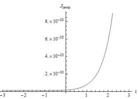
𝐽_{𝑙𝑒𝑤𝑎𝑡}= ^𝑖ℏ

2𝑚(Ѱ^{(𝑟𝑒𝑔)}(𝑥, 𝑅(𝑡))

𝑙𝑒𝑤𝑎𝑡

𝑑Ѱ^{(𝑟𝑒𝑔)∗}(𝑥,𝑅(𝑡))_{𝑙𝑒𝑤𝑎𝑡}

𝑑𝑥 − Ѱ^{(𝑟𝑒𝑔)∗}(𝑥, 𝑅(𝑡))

𝑙𝑒𝑤𝑎𝑡

Ѱ^{(𝑟𝑒𝑔)}(𝑥,𝑅(𝑡))_{𝑙𝑒𝑤𝑎𝑡}

𝑑𝑥 ) (17)

(8)

The reflection coefficient (𝑅) and transmission coefficient (𝑇) can be calculated.(𝑅)(𝑇) 𝑅 =^|𝐽^{𝑝𝑎𝑛𝑡𝑢𝑙}^|

|𝐽_{𝑚𝑎𝑠𝑢𝑘}| (18)

𝑅 = ^|𝐽^{𝑙𝑒𝑤𝑎𝑡}^|

|𝐽_{𝑚𝑎𝑠𝑢𝑘}| (19)

Bound State (E<0)

The potential Schrödinger equation of the delta function in the bound state becomes:

𝑑²𝜓 𝑑𝑥² = −^2𝑚

ħ² 𝐸𝜓 = 𝜅²𝜓 (20)

The wave function in the bound state or E < 0 for the delta function potential is:

Ѱ₁(𝑥, 𝑡) = 𝐴𝑒^{−(𝜅𝑥+𝑖𝜔𝑡)}+ 𝐵𝑒^{(𝜅𝑥−𝑖𝜔𝑡)}, for (𝑥 < 0) (21)

Ѱ₂(𝑥, 𝑡) = 𝐹𝑒^{−(𝜅𝑥+𝑖𝜔𝑡)}+ 𝐺𝑒^{(𝜅𝑥−𝑖𝜔𝑡)}, for (𝑥 > 0) (22) G becomes worth zero. Until the equations (21) and (22) become as follows :

Ѱ1(𝑥, 𝑡) = 𝐵𝑒^{(𝜅𝑥−𝑖𝜔𝑡)}, for (𝑥 < 0) (23)

Ѱ₂(𝑥, 𝑡) = 𝐹𝑒^{−(𝜅𝑥+𝑖𝜔𝑡)}, for (𝑥 > 0) (24)

Equations (23) and (24) representing the bound state of the delta function (E<0) can be described as figure 2 below:

Figure 2. Bound state (E<0) on the delta function (Griffits, 2005:72) Based on these conditions obtainedF =B, so that:

Ѱ(𝑥, 𝑡) = {𝐵𝑒^{(𝜅𝑥−𝑖𝜔𝑡)} 𝐵𝑒^{−(𝜅𝑥+𝑖𝜔𝑡)}

untuk (𝑥 < 0)

untuk (𝑥 > 0) (25)

 = ⁻2mE (26)

Therefore, normalizations of equations (23) and (24) to obtain the constants F and B byn give a limit -∞ up to ∞∞∞. The normalization formula can be written as follows:

∫ |Ѱ(𝑥, 𝑡)|_−∞^∞ ²𝑑𝑥 = 1 (27) Substitute equations (23) and (24) into the normalized formula for equation (27), so that it becomes:

∫ (𝐵𝑒_−∞⁰ ^{(𝜅𝑥−𝑖𝜔𝑡)})(𝐵𝑒^{(𝜅𝑥+𝑖𝜔𝑡)})𝑑𝑥 +∫ (𝐹𝑒₀^∞ ^{−(𝜅𝑥+𝑖𝜔𝑡)})(𝐹𝑒^{−(𝜅𝑥−𝑖𝜔𝑡)})𝑑𝑥 = 1 (28)

(9)

So that the value of the constant F is obtained, namely:

𝐹 = √𝜅 (29)

Substituting the value of the constant B into the potential wave equation of the delta state function is bound to equations (23) and (24), so it can be written as follows:

Ѱ1(𝑥, 𝑡) = 𝐵𝑒^{(𝜅𝑥−𝑖𝜔𝑡)} =√𝜅𝑒^{(𝜅𝑥−𝑖𝜔𝑡)} (30)

Ѱ2(𝑥, 𝑡) = 𝐹𝑒^{−(𝜅𝑥+𝑖𝜔𝑡)}=√𝜅𝑒^{−(𝜅𝑥+𝑖𝜔𝑡)} (31)

The regularization phase (𝜃₁) value can be calculated by substituting the position- dependent wave function 𝜓₁ in equation (30) to equation (10) and 𝜃₂ can be calculated by substituting the position-dependent wave function 𝜓₂ in equation (31) to equation (10). (𝜃₁)𝜓₁ 𝜃₂𝜓₂

𝜓1= √𝜅𝑒^(𝜅𝑥) (32)

𝜓₂= √𝜅𝑒^{−(𝜅𝑥)} (33)

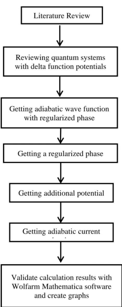
𝜃1= ^𝐴¹

−2𝜅²𝑒^−2𝜅𝑥 (34)

Equation (34) can be described in grafik form with input as shown 3 below:

Figure 3 Input equation (34) for the graph figure 4

Figure 4 Regularization Phase graph at E <0 state with(x < 0)

Figure 4 above shows that when x = -1 m, 𝜃₁ = -4 and when x is positive 𝜃₁ it gets closer to zero. K ethics value x is negative then the value of the regularization phase is negative too, with the greater the value of x the greater the value of the regularization phase.cut the x-axis. Value 𝐴1 is a constant so it is assumed with 1.

𝜃₂= ^𝐴¹

2𝜅²𝑒^2𝜅𝑥 (35)

(10)

Equation (35) can be described in graphic form with inputs such as figure 5 as follows:

Figure 5 Input equation (35) for the graph figure 6

Figure 6 Regularization Phase graph at state E<0 with(x > 0)

Figure 6 above shows that when x = 1 m, 𝜃₂ = 4 and x is negative the value 𝜃₂

gets closer to zero. K x value is directly proportional to the value of the regularization phase, the greater the value of x, the greater the value of the regularization phase.

The regularization phase will be worth infinitely and worth 𝑥 → +∞ towards zero when𝑥 → −∞. Figure 6 above is an exponential graph.

Based on the regularization phase value obtained, the adiabatic wave function is obtained through substituting the regularization phase value in equations (34) and (35) to equation (6) and can be written as follows:

Ѱ₁^{(𝑟𝑒𝑔)}(𝑥, 𝑅(𝑡)) = √𝜅𝑒^(𝜅𝑥)𝑒^{−(𝑖 ℏ}^{⁄ ) ∫ 𝐸}^𝑛^{(𝑅(𝑡)) 𝑑𝑡}

𝑡

0 𝑒^𝑖𝜀^−2𝜅2^𝐴1 ^𝑒^−2𝜅𝑥Ѱ₁^{(𝑟𝑒𝑔)}(𝑥, 𝑅(𝑡)) = √𝜅𝑒^(𝜅𝑥)𝑒^{−(𝑖 ℏ}^{⁄ ) ∫ 𝐸}^𝑛^{(𝑅(𝑡)) 𝑑𝑡}

𝑡

0 𝑒^𝑖𝜀^−2𝜅2^𝐴1 ^𝑒^−2𝜅𝑥 (36)

Ѱ2(𝑟𝑒𝑔)

(𝑥, 𝑅(𝑡)) = √𝜅𝑒^{(−𝜅𝑥)}𝑒^{−(𝑖 ℏ}^{⁄ ) ∫ 𝐸}^𝑛^{(𝑅(𝑡)) 𝑑𝑡}

𝑡

0 𝑒^𝑖𝜀^2𝜅2^𝐴1^𝑒^2𝜅𝑥 (37) Ѱ2(𝑟𝑒𝑔)

(𝑥, 𝑅(𝑡)) = √𝜅𝑒^{(−𝜅𝑥)}𝑒^{−(𝑖 ℏ}^{⁄ ) ∫ 𝐸}^𝑛^{(𝑅(𝑡)) 𝑑𝑡}

𝑡

0 𝑒^𝑖𝜀^2𝜅2^𝐴1^𝑒^2𝜅𝑥

The equation above can be seen in graphic form by calculating the amplitude value of each wave, with the following formula:

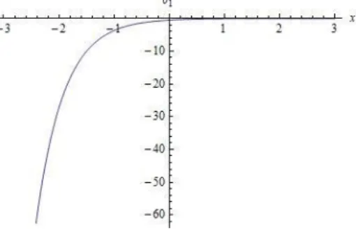
|Ѱ1(𝑟𝑒𝑔)(𝑥, 𝑅(𝑡))²| = (𝜅𝑒^2𝜅𝑥) (38) Until when depicted in graphic form with inputs such as the following 77 pictures :

(11)

Figure 7 Input wave amplitude (equation 38) for the graph in figure 8

Figure 8. Amplitude graph for x 0 in case E < 0<

Figure 8 above is illustrated with the value 𝜅 = 1, and the value x from -3 to 0. From the graph above it can be seen that when x = 0 the wave function is equal to 𝜅 . The smaller the value of x, the wave function is closer to 0, when x is equal to -∞ the wave function is 0. The function graph above is an uphill exponential function graph that has the characteristics of never intersecting the x-axis.

The amplitude graph for the regularized wave function at x > 0 bound state is as follows:

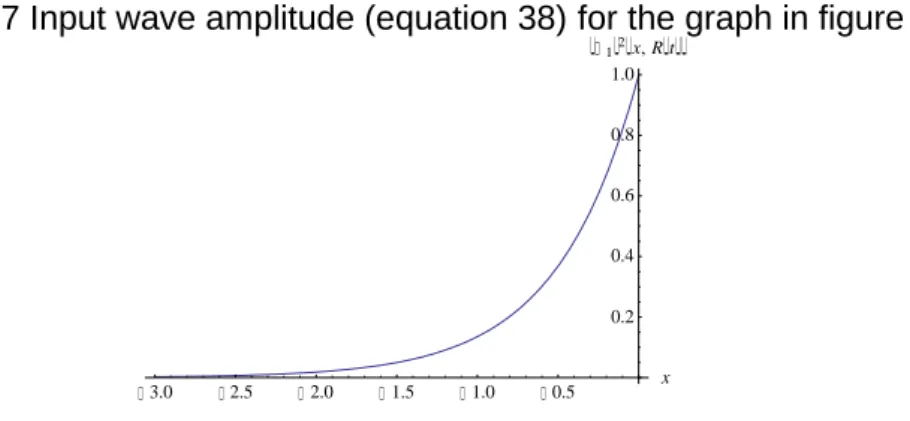
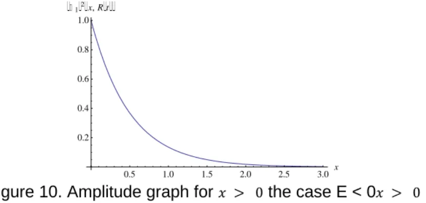
|Ѱ2(𝑟𝑒𝑔)(𝑥, 𝑅(𝑡))|²= (𝜅𝑒^−2𝜅𝑥) (39)

Equation (39) can be described in graphic form with inputs such as figure 9 below:

Figure 9 Input wave amplitude (equationn 39) for the graph in figure 10

Figure 10. Amplitude graph for 𝑥 > 0 the case E < 0𝑥 > 0

Figure 1 0 above is illustrated with the value of 𝜅 = 1 m^-1 andx value from 0 to 3 m. From the graph above it can be seen that when x = 0 m the wave function is equal to 𝜅. The wave function sgets smaller the smaller the x gets, when x equals +∞ the wave function is 0.∞ The function graph above is a graph of a descending exponential function that never intersects the x-axis.

3.0 2.5 2.0 1.5 1.0 0.5 x

0.2 0.4 0.6 0.8 1.0 12x,R t

0.5 1.0 1.5 2.0 2.5 3.0 x

0.2 0.4 0.6 0.8 1.0 12

x,R t

(12)

Additional potentials can be calculated (𝑉̃) by substituting position-dependent wave functions 𝜓₁ and 𝜓₂ into equation (12). As shown in equation (12), if the wave function is real, the additional potential (𝑉̃) is zero. So it is written in the equation to be:(𝑉̃)

𝑉̃₁= 0 (40)

𝑉̃2= 0 (41)

In the bound state 𝐸 < 0 , there are only two currents, namely the reflected current

(𝐽_{𝑝𝑎𝑛𝑡𝑢𝑙})and the passing current (𝐽_{𝑙𝑒𝑤𝑎𝑡}).𝐸 < 0(𝐽_{𝑝𝑎𝑛𝑡𝑢𝑙})(𝐽_{𝑙𝑒𝑤𝑎𝑡}) Ѱ^{(𝑟𝑒𝑔)}(𝑥, 𝑅(𝑡))

𝑝𝑎𝑛𝑡𝑢𝑙 = 𝐵𝑒^{(𝜅𝑥−𝑖𝜔𝑡)}e^ⅈεθ¹^(x,t) (42) Ѱ^{(𝑟𝑒𝑔)}(𝑥, 𝑅(𝑡))_{𝑙𝑒𝑤𝑎𝑡}= 𝐹𝑒^{−(𝜅𝑥+𝑖𝜔𝑡)}e^ⅈεθ²^(x,t) (43) The density of the reflected current can be calculated using equation (16) so that:

The derivative 𝜃1 can be calculated so as to produce:

𝑑𝜃₁ 𝑑𝑥 =^𝑑

𝐴1

−2𝜅2 𝑒^−2𝜅𝑥

𝑑𝑥 =^𝐴1

𝜅 𝑒^−2𝜅𝑥 (44)

The derivative Ѱ^{(𝑟𝑒𝑔)}(𝑥, 𝑅(𝑡))

𝑝𝑎𝑛𝑡𝑢𝑙 can be calculated so as to produce:

𝑑Ѱ^{(𝑟𝑒𝑔)}(𝑥,𝑅(𝑡))_{𝑝𝑎𝑛𝑡𝑢𝑙}

𝑑𝑥 = 𝐵 (𝜅 + iε^𝐴1

𝜅 𝑒^−2𝜅𝑥) 𝑒^{(𝜅𝑥−𝑖𝜔𝑡)}e^ⅈεθ¹^(x,t) (45) The derivative Ѱ^{(𝑟𝑒𝑔)∗}(𝑥, 𝑅(𝑡))_{𝑝𝑎𝑛𝑡𝑢𝑙} can be calculated so as to produce:

𝑑Ѱ^{(𝑟𝑒𝑔)∗}(𝑥,𝑅(𝑡))_{𝑝𝑎𝑛𝑡𝑢𝑙}

𝑑𝑥 = 𝐵 (𝜅 + iε^𝐴1

𝜅 𝑒^−2𝜅𝑥) 𝑒^{(𝜅𝑥−𝑖𝜔𝑡)}e^ⅈεθ¹^(x,t) (46)

Substituting the derivative products in equations (44), (45), and (46) into equation (16) so that 𝐽𝑝𝑎𝑛𝑡𝑢𝑙 the value is as follows:

𝐽𝑝𝑎𝑛𝑡𝑢𝑙= ^ℏ

𝑚(|𝐵|²(ε^𝐴1

𝜅 𝑒^−2𝜅𝑥) ) (47)

Equation (47) can be depicted in graphic form with inputs such as figure 11 below:

Figure 11 Input equation (47) for the graph in figure 12

(13)

Figure 12 Graph of Bounce Current Meeting in case E < 0

Figure 12 above shows that when the density value of the reflected current goes towards zero when the 𝑥 → +∞ current density value goes to infinity. 𝑥 → −∞ x then the density value of the reflected current is getting closer to zero. When x = -1 m the bounce current density is 0.5 × 10⁻³³ A/m², and when× 10⁻³³ x is positive the bounce current density is close to zero. The density value of the reflected current is inversely proportional to the value of x. Figure 2 is a graph of the descending exponential function.

The density of the current can be calculated using equation (17) so that : The derivative Ѱ^{(𝑟𝑒𝑔)}(𝑥, 𝑅(𝑡))

𝑙𝑒𝑤𝑎𝑡 can be calculated so as to produce:

^𝑑Ѱ

(𝑟𝑒𝑔)(𝑥,𝑅(𝑡))_{𝑙𝑒𝑤𝑎𝑡}

𝑑𝑥 = 𝐹 (−𝜅 + 𝑖ε^𝐴1

𝜅 𝑒^2𝜅𝑥) 𝑒^{−(𝜅𝑥+𝑖𝜔𝑡)}e^ⅈεθ²^(x,t) (48) The derivative Ѱ^{(𝑟𝑒𝑔)∗}(𝑥, 𝑅(𝑡))_{𝑙𝑒𝑤𝑎𝑡} can be calculated so as to produce:

𝑑𝐹Ѱ^{(𝑟𝑒𝑔)∗}(𝑥,𝑅(𝑡))_{𝑙𝑒𝑤𝑎𝑡}

𝑑𝑥 = 𝐹 (𝜅 − 𝑖ε^𝐴1

𝜅 𝑒^2𝜅𝑥 ) 𝑒^{(𝜅𝑥+𝑖𝜔𝑡)}e^−ⅈε𝜃²^(x,t) (49) The derivative 𝜃₂ can be calculated so as to produce:

𝑑𝜃₂ 𝑑𝑥 =^𝑑

𝐴1 2𝜅2 𝑒^2𝜅𝑥

𝑑𝑥 =^𝐴1

𝜅 𝑒^2𝜅𝑥 (50)

Substitution of the derivative results in equations (48), (49), and (50) to equation (16) so that the value is as follows:𝐽𝑙𝑒𝑤𝑎𝑡

𝐽_{𝑙𝑒𝑤𝑎𝑡}= ^ℏ

𝑚(|𝐹|²(𝑖𝜅 + ε^𝐴1

𝜅 𝑒^2𝜅𝑥 ) ) (51)

(14)

Figure 14 Graph of Passing Current Meeting in case E < 0

Figure 14 shows that the density of the current is directly proportional to x, the density of the current increases with the increase of x. When x = 1 m of current density is 0.5, × 10⁻³³ A/m² and when x is negative the current density is close to zero where x to the density of the current through is infinite. 𝑥 → +∞ The chart above is an uphill exponential graph.

Scatter State (E>0)

In the scattering state, the Schrödinger equation can be written as follows:

𝑑²𝜓 𝑑𝑥² = −^2m

ħ² 𝐸𝜓 = −𝑘²𝜓 (52)

The wave function in the bound state or E > 0 for the delta function potential is:

Ѱ₁(𝑥, 𝑡) = 𝐴 𝑒^{𝑖(𝑘𝑥−𝜔𝑡)}+ 𝐵𝑒^{−𝑖(𝑘𝑥+𝜔𝑡)}for (𝑥 < 0) (53) Ѱ₂(𝑥, 𝑡) = 𝐹 𝑒^{𝑖(𝑘𝑥−𝜔𝑡)}+ 𝐺𝑒^{−𝑖(𝑘𝑥+𝜔𝑡)}for (𝑥 > 0) (54) Since G is 0, the equation (54) becomes:

Ѱ₂(𝑥, 𝑡) = 𝐹𝑒^{𝑖(𝑘𝑥−𝜔𝑡)} for (𝑥 > 0) (55)

𝑘 =^√2𝑚𝐸_ħ (56)

Equations (53) and (55) can be described in graphic form as shown 15 below :

Figure 15 Scattering state (E>0) on delta function potential (Griffits, 2005:72) By using the properties of continuity Ѱ₁(𝑥, 𝑡) and Ѱ₂(𝑥, 𝑡) at the moment𝑥 = 0Ѱ₁(𝑥, 𝑡)Ѱ₂(𝑥, 𝑡)𝑥 = 0. So it can be written as follows:

(𝐴 + 𝐵) = (𝐹 + 𝐺) (57)

(15)

The derivative of Ѱ₁(𝑥, 𝑡) and ^Ѱ²^{(𝑥, 𝑡)} at the time of x = 0 is:^Ѱ¹^{(𝑥, 𝑡)Ѱ}²^{(𝑥, 𝑡)}

𝜕

𝜕𝑥Ѱ₁(𝑥, 𝑡) = ^𝜕

𝜕𝑥Ѱ₂(𝑥, 𝑡) (58)

∆^𝜕Ѱ

𝜕𝑥 = 𝑖𝑘(𝐹 − 𝐺 − 𝐴 + 𝐵) (59)

By looking at the equation ∆ (^𝜕Ѱ

𝜕𝑥) = −^2𝑚𝛼

ħ² Ѱ(0). Then the above equation can be changed to:

𝑖𝑘(𝐹 − 𝐺 − 𝐴 + 𝐵) = −^2𝑚𝛼

ħ² (𝐴 + 𝐵) (60)

𝐹 − 𝐺 = 𝐴 (^{2𝑖𝑚𝛼}

ħ²𝑘 + 1) − 𝐵 (^{−2𝑖𝑚𝛼}

ħ²𝑘 + 1) with 𝛽 = ^𝑚𝛼

ħ²𝑘 (61) 𝐹 − 𝐺 = 𝐴(1 + 2𝑖𝛽) − 𝐵(1 − 2𝑖𝛽) (62) To find the value of B Substitution of equation (62) to equation (57)

𝐵 = 𝐴_{(1−𝑖𝛽)}^(𝑖𝛽) (63)

𝐹 = 𝐴 ( ¹

(1−𝑖𝛽)) (64)

Evidenced by the normalization of wave functions in equations (53) and (54) by being limited from -∞ to ∞ those that produce infinite values.

∫ |Ѱ(𝑥, 𝑡)|_−∞^∞ ²𝑑𝑥 = 1 (65)

∫ |Ѱ_−∞⁰ 1(𝑥, 𝑡)|²𝑑𝑥 +∫ |Ѱ₀^∞ 2(𝑥, 𝑡)|²𝑑𝑥 = 1 (66)

∫ (Ѱ₀^∞ 2(𝑥, 𝑡))(Ѱ₂(𝑥, 𝑡))^∗𝑑𝑥 = 1

∫ (Ѱ_−∞⁰ 1(𝑥, 𝑡))(Ѱ₁(𝑥, 𝑡))^∗ 𝑑𝑥 +∫ (Ѱ₀^∞ 2(𝑥, 𝑡))(Ѱ₂(𝑥, 𝑡))^∗𝑑𝑥 = 1 (67 & 68)

∫ (𝐴𝑒_−∞⁰ ^{𝑖(𝑘𝑥−𝜔𝑡)}+ 𝐵𝑒^{−𝑖(𝑘𝑥+𝜔𝑡)})(𝐴𝑒^{−𝑖(𝑘𝑥−𝜔𝑡)}+ 𝐵𝑒^{𝑖(𝑘𝑥+𝜔𝑡)})𝑑𝑥+ ∫ (𝐹𝑒₀^∞ ^{𝑖(𝑘𝑥−𝜔𝑡)})(𝐹𝑒^{−𝑖(𝑘𝑥−𝜔𝑡)})𝑑𝑥 = 1

Substitute equations (63) and (64) to equations (53) and (54) so that a wave function is obtained in the scattering state, which is as follows:

Ѱ₁(𝑥, 𝑡) = 𝐴 𝑒^{𝑖(𝑘𝑥−𝜔𝑡)}+ 𝐴 ^(𝑖𝛽)

(1−𝑖𝛽) 𝑒^{−𝑖(𝑘𝑥+𝜔𝑡)} (69) Ѱ₂(𝑥, 𝑡) = 𝐴 ( ¹

(1−𝑖𝛽)) 𝑒^{𝑖(𝑘𝑥−𝜔𝑡)} (70)

The regularization phase (𝜃₁) value can be calculated by substituting the position-dependent wave function 𝜓₁ in equation (69) to equation (11) and 𝜃₂ can be calculated by substituting the position-dependent wave function 𝜓₂ in equation (31) to equation (11). (𝜃₁)𝜓₁ 𝜃₂𝜓₂

𝜓₁= 𝐴 𝑒^𝑖⁽^𝑘𝑥⁾+ 𝐴₍_1−𝑖𝛽⁽^𝑖𝛽⁾₎𝑒^−𝑖⁽^𝑘𝑥⁾ (71)

𝜓₂= 𝐴( ¹

(1−𝑖𝛽)) 𝑒^𝑖⁽^𝑘𝑥⁾ (72)

𝜃₁ = ^𝐴¹^𝑥

𝐴²(1+_(1+𝑖𝛽)^{(−𝑖𝛽)}𝑒^{2𝑖𝑘𝑥}+_{(1−𝑖𝛽)}^(𝑖𝛽) 𝑒^{−2𝑖𝑘𝑥}+ ^(𝛽2) (1+𝛽2))

(73)

Equation (73) can be described in graphic form with inputs such as figure 16

(16)

Figure 17 Regularization Phase at E>0 with (x < 0)

Figure 17 shows that the regularization phase hitsa satellite dish every 3 m.

𝜃₂ = ^𝐴²^𝑥(1+𝛽²⁾

𝐴² (74)

Figure 19 Regularization Phase Graph at E>0 with (x > 0)

Figure 19 above shows that the value of the regularization phase at E>0 is

(x > 0) directly proportional to the value of x, the greater the value of x, the greater the regularization phase. The gradient above is a liear graph.

The adiabatic wave function is obtained through substituting the regularization phase value in equations (73) and (74) to equation (5) and can be written as follows:

(17)

e

ⅈε ^A1x

A2(1+(−iβ)

(1+iβ)e2ikx+ (iβ)

(1−iβ)e−2ikx+ (β2) (1+β2))

(75)

Ѱ₂^{(𝑟𝑒𝑔)}(𝑥, 𝑅(𝑡)) = 𝐴 ( ¹

(1−𝑖𝛽)) 𝑒^{𝑖(𝑘𝑥)} 𝑒^{−(𝑖 ℏ}^{⁄ ) ∫ 𝐸}^𝑛^{(𝑅(𝑡)) 𝑑𝑡}

𝑡

0 𝑒^𝑖𝜀^{𝐴2𝑥(1+𝛽2)}^𝐴2 Ѱ₂^{(𝑟𝑒𝑔)}(𝑥, 𝑅(𝑡)) = 𝐴 ( ¹

(1−𝑖𝛽)) 𝑒^{𝑖(𝑘𝑥)} 𝑒^{−(𝑖 ℏ}^{⁄ ) ∫ 𝐸}^𝑛^{(𝑅(𝑡)) 𝑑𝑡}

𝑡

0 𝑒^𝑖𝜀^{𝐴2𝑥(1+𝛽2)}^𝐴2 (76) Equation (75) above can be seen in graph form by calculating the amplitude value of each wave, with the following formula:

|Ѱ₁^{(𝑟𝑒𝑔)}(𝑥, 𝑅(𝑡))²| =𝐴²(1 +₍⁽_1+𝑖𝛽^−𝑖𝛽⁾₎𝑒^{2𝑖𝑘𝑥}+₍_1−𝑖𝛽⁽^𝑖𝛽⁾₎𝑒^{−2𝑖𝑘𝑥}+ ⁽^𝛽

2)

(1+𝛽²)) (77)

Equation (77) can be described in graphform with inputs such as figure 2020 below:

Figure 21. 2-dimensional graph of the amplitudo of the wave function of the scattering state (E > 0) at x < 0 by k = 1

Figure 21 above is depicted with values 𝛽 = 1, k = 1 m^-1, 𝛽 = 1A = 1, and x from -5 to 5 m. When x = -2 m the wave reaches the maximum value of 2.9 m and when x = -3.5 m the wave reaches the minimum value of 0.1 m. It can be seenthat the

(18)

gelomba ng is formed only a little but the wavelength is large. The value of k is directly proportional to the wavelength but inversely proportional to the many waves.

Figure 23. 2-dimensional graph of the amplitudo of the wave function of the scattering state (E > 0) at x < 0 with k = 3

Figure 23 above is depicted with values 𝛽 = 1, k =3 m^-1, 𝛽 = 1A = 1, and x from -5 m to 5 m. You can see more waves than figure 19. The higher the k, the more waves formed. The lower the k, the fewer waves formed. Many waves are formed inversely proportional to k.

Equation (77) can be depicted in the form of a 3-dimensional graph with inputssuch as figure 24 below:

Figure 25 3-dimensional graph of the amplitudo wave function to the scattering form (E > 0) at x <0

(19)

Figure 25 above is illustrated with 𝛽= 1, A = 1, x from -5 to 5𝛽, and k from -1 to 1.

The amplitude graph for the regularized wave function at x0 ≥scattering state is as follows:

|Ѱ₂^{(𝑟𝑒𝑔)}(𝑥, 𝑅(𝑡))|²=𝐴²( ¹

(1+𝛽²)) (78)

up to the equation (78) when depicted in the form of a 2-dimensional graphic with inputs such as the following picture 26 :

Figure 24 Input amplitude of the wave (perequation 78) graph in figure 27

Figure 25. 2-dimensional graph of the amplitudo of the wave function of the scattering state (E>0) at x > 0

Figure 27 above is illustrated with the value 𝛽 = 1, 𝛽 = 1and the value A from - 5 m to 5 m. It can be seen that at A = -5 and 5 the wave function is of enormous value even towards infinity. Whereas when A approaches 0 the wave function goes to zero. The graph above is a parabolic graph.

Equation (78) when depicted in the form of a 3-dimensional graph with input can be seen as figure 28 below:

(20)

Figure 27. 3-dimensional graph of the amplitude of the scattering state wave function (E>0) at x > 0 when x and A are varied

Figure 29 above is illustrated with 𝛽 = 1, x from -5 to 5 𝛽 = 1m, and A from -1 to 1. It can be seen that when A = -1 and 1 the wave function goes to infinity, while when A approaches zero the wave function goes to zero.

Equation (78) when depicted in the form of a 3-dimensional graph with x and t varied with input can be seen as figure 30 below:

Figure 30 Input equation (78) for the graph in figure 31

Figure 31 Graphic amplitudo wave function on x≥0 scattering state

Figure 3 1 above is illustrated with 𝛽 =1, k = 1 m^-1, 𝛽𝜔 = 1 rad/s, A = 1, x from -5 to 5 m, and t𝜔 = 1 from -1 to 1. The wave function is constant even if the variables x and t are changed.

Additional potentials can be calculated (𝑉̃) by substituting position-dependent wave functions in equation (71) and in equation (72) to equation (13). The wave function depends on position 𝜓₁𝜓₂𝜓₁ and 𝜓₂ is imaginary so it is written in the equation to be:

𝑑𝜓₁

𝑑𝑥 = (𝐴𝑖𝑘 𝑒^{𝑖(𝑘𝑥)}− 𝐴 ^(𝑖𝛽)

(1−𝑖𝛽)𝑖𝑘𝑒^{−𝑖(𝑘𝑥)}) (79)

𝑑𝜃₁ 𝑑𝑥 = ^𝑑

𝑑𝑥

𝐴₁𝑥

𝐴²(1+_(1+𝑖𝛽)^{(−𝑖𝛽)}𝑒^{2𝑖𝑘𝑥}+_{(1−𝑖𝛽)}^(𝑖𝛽) 𝑒^{−2𝑖𝑘𝑥}+ ^(𝛽2) (1+𝛽2))