Reinforcement learning algorithms with function approximation: Recent advances and applications
Xin Xu
⇑, Lei Zuo, Zhenhua Huang
College of Mechatronics and Automation, National University of Defense Technology, Changsha 410073, PR China
a r t i c l e i n f o
Article history:
Received 19 June 2012
Received in revised form 30 June 2013 Accepted 17 August 2013
Available online 5 September 2013
Keywords:
Reinforcement learning Function approximation
Approximate dynamic programming Learning control
Generalization
a b s t r a c t
In recent years, the research on reinforcement learning (RL) has focused on function approximation in learning prediction and control of Markov decision processes (MDPs).
The usage of function approximation techniques in RL will be essential to deal with MDPs with large or continuous state and action spaces. In this paper, a comprehensive survey is given on recent developments in RL algorithms with function approximation. From a the- oretical point of view, the convergence and feature representation of RL algorithms are analyzed. From an empirical aspect, the performance of different RL algorithms was eval- uated and compared in several benchmark learning prediction and learning control tasks.
The applications of RL with function approximation are also discussed. At last, future works on RL with function approximation are suggested.
Ó2013 Elsevier Inc. All rights reserved.
1. Introduction
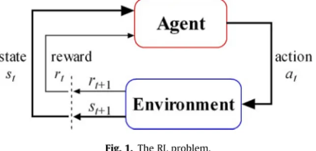
Reinforcement learning (RL) is a machine learning framework for solving sequential decision problems that can be mod- eled as Markov Decision Processes (MDPs). In recent years, RL has been widely studied not only in the machine learning and neural network community but also in operations research and control theory[28,70,71,93,111,120,134,141]. In reinforce- ment learning, the learning agent interacts with an initially unknown environment and modifies its action policies to maximize its cumulative payoffs. Thus, RL provides an efficient framework to solve learning control problems which are dif- ficult or even impossible for supervised learning and traditional dynamic programming (DP) methods. The aim of dynamic programming is to compute optimal policies given a perfect model of the environment as an MDP. Classical DP algorithms have some limitations both due to their assumption of a perfect model and due to their great computational costs. In fact, RL methods can be viewed as adaptive DP or approximate DP, with less computation and without assuming a perfect model of the environment[111]. From the perspective of automatic control, the DP/RL framework comprises a nonlinear and stochas- tic optimal control problem[29]. Moreover, RL is an important way for adaptive optimal control[18,112]. In the research of human brain, RL has been studied as an important mechanism for human learning[113,137–139]. From the viewpoint of artificial intelligence, RL is a basic mechanism for an agent to optimize its behavior in an uncertain environment [28,121,135,140].Fig. 1illustrates the main components of the RL problem, where an agent receives the state and reward information at timet, takes action at to make the environment’s state change to next statest+1with a reward rt+1. The learning objective is to find an action policy to optimize the long-term expected total or average reward from the environment.
0020-0255/$ - see front matterÓ2013 Elsevier Inc. All rights reserved.
http://dx.doi.org/10.1016/j.ins.2013.08.037
⇑Corresponding author. Tel.: +86 731 84574980.
E-mail addresses:[email protected],[email protected](X. Xu).
Contents lists available atScienceDirect
Information Sciences
j o u r n a l h o m e p a g e : w w w . e l s e v i e r . c o m / l o c a t e / i n s
Function approximation has been a traditional topic in the research of machine learning. In earlier works, researchers mainly focused on function approximation techniques for supervised learning problems which can be formulated as a regression task[28]. For a regression task, the training samples are in the form of input–output pairs (xi,yi),i= 1, 2,. . .,n.
The regression problem can be stated as: given a training data setD=f(yi;ti),i= 1, 2,. . .,n, of input vectorsyiand associated targetsti, the goal is to find a functiong(y) which approximates the relation inherited between the data set points and it can be used to infer the outputtfor a new input data pointy. Generally, a regression algorithm has a loss functionL(t;g(y)), which describes how the estimated function deviated from the true one. Many forms for the loss function have been pro- posed in the literature: e.g. linear, quadratic loss function, exponential, etc.[72].
To compute the optimal or near-optimal policies of MDPs, RL algorithms usually estimate the value functions of MDPs by observing data generated from state transitions. However, since no explicit teacher signals can be obtained in RL, the estimation of value functions is different from the function regression problem in supervised learning. In earlier research of RL, tabular algorithms were popularly studied, such as tabular Q-learning and tabular Sarsa-learning. In tabular RL algorithms, value func- tions are represented and estimated in tabular forms for each state or state-action pair. But in many real-world applications, a learning controller has to deal with MDPs with large or continuous state and action spaces. In such cases, earlier RL algorithms such as Q-learning and Sarsa-learning usually converge slowly when tabular representations of value functions are used. Since function approximation is essential to realize the generalization ability of learning machines, function approximation and gen- eralization methods for RL have received more and more research interests in recent years[14,31,44,45,114,124,125,133,153].
Currently, there are three main categories of research work on RL methods with function approximation, i.e., policy search[9], value function approximation (VFA)[11], and actor–critic methods[13,16]. Among these three classes of approximate RL meth- ods, the actor–critic algorithms, viewed as a hybrid of VFA and policy search, have been shown to be more effective than VFA or policy search in online learning control tasks with continuous spaces[95]. In an actor–critic learning control architecture, there is an actor for policy learning and a critic for value function approximation or policy evaluation. The policy evaluation process in the critic is also called learning prediction, which can be viewed as a sub-problem of RL.
In the past decade, the research works on RL with function approximation have been brought together with the approx- imate dynamic programming (ADP) community[93,134], which is to compute near-optimal solutions to MDPs with large or continuous spaces. One common objective of ADP and RL is to solve MDPs with large or continuous state and action spaces.
Thus, RL and ADP provide a very promising framework for learning control problems which are difficult or even impossible for supervised learning and mathematical programming methods. Originally, RL methods mainly focused on learning control problems in MDPs without model information while ADP methods usually approximate near-optimal solutions of MDPs with some model information, which can be viewed as planning cases for sequential decision making. In this paper, we will mainly focus on recent developments in RL algorithms with function approximation and related works on ADP algorithms with function approximation will also be surveyed. Firstly, since learning prediction is an important sub-problem of RL, ma- jor advances in learning prediction algorithms with function approximation are discussed. Specifically, we put more empha- sis on the developments in temporal-difference (TD) learning theory and algorithms, which are basic mechanisms for value function approximation. Secondly, learning control algorithms with function approximation are surveyed, where the main focus is put on highly efficient RL algorithms with function approximation such as fitted-Q iteration, approximate policy iter- ation, and adaptive critic designs (ACDs). The convergence of RL algorithms with different representations is analyzed from a theoretical point of view. Furthermore, the performance of different RL algorithms was evaluated and compared in several benchmark learning prediction and learning control tasks. The selected RL algorithms for performance comparisons have been popularly studied in the literature and most of them are state-of-the-art RL approaches with function approximation.
The applications of RL will also be summarized by analyzing the advantages and disadvantages of different RL algorithms.
The rest of this paper is organized as follows. In Section2, an overview on RL algorithms with function approximation for learning prediction is given. The RL methods with function approximation for learning control in MDPs are introduced in Section3. Then, the theoretical results on the convergence of RL algorithms with function approximation are discussed in Section4. The performance of different RL algorithms with function approximation was evaluated and compared in Section5.
In Section6, the applications of RL are summarized, where the advantages and disadvantages of different algorithms are highlighted. Section7discusses some open problems in function approximation of RL. In the end, Section8draws conclu- sions and suggests future work.
Fig. 1.The RL problem.
2. RL algorithms with function approximation for learning prediction
In RL, there are two basic tasks. One is called learning prediction and the other is called learning control. The goal of learn- ing control is to estimate the optimal policy or optimal value function of an MDP without knowing its complete model.
Learning prediction aims to solve the policy evaluation problem of a stationary-policy MDP, which can also be viewed as a Markov reward process, without prior model information and it can be regarded as a sub-problem of learning control. Fur- thermore, in RL, learning prediction is different from that in supervised learning[14]. As pointed out by Sutton[111,114], the prediction problems in supervised learning are single-step prediction problems while those in reinforcement learning are multi-step prediction problems. To solve multi-step prediction problems, a learning system must predict outcomes that de- pend on a future sequence of decisions[142]. Therefore, the theory and algorithms for multi-step learning prediction become an important topic in RL and much research work has been done in the literature[114,124]. In this section, we will focus on learning prediction methods with function approximation. At first, some introduction on the Markov reward process model for learning prediction is given.
2.1. Markov reward process
Markov reward processes are popular stochastic models for sequential modeling and decision making. A Markov reward process can be modeled as a tuple {X,R,P}, whereXis the state space,Ris the reward function,Pis the state transition prob- ability. Let {xtjt= 0, 1, 2,. . .;xt2X} denote a state sequence generated by a Markov reward process. For each state transition fromxttoxt+1, a scalar rewardrtis defined. The state transition probabilities satisfy the following property:
Pfxtþ1jxt;xt1;. . .;x1;x0g ¼Pfxtþ1jxtg ð1Þ
Let the trajectory generated by the Markov chain be denoted by {xtjt= 0, 1, 2,. . .,xt2X}.The dynamics of the Markov chain can be described by a transition probability matrixPwhose (i,j)th entry, denoted bypij, is the transition probability forxt+1=jgiven thatxt=i. For each state transition fromxttoxt+1, a scalar rewardrtis defined. The expected average reward or value starting from a statexis defined as:
q
ðxÞ ¼limN!1
1 NE XN
t¼0
rtþ1
x0¼x
" #
ð2Þ
For the discounted case, the value function of each state is defined as follows:
VðxÞ ¼E X1
t¼0
c
trtþ1x0¼x
( )
ð3Þ where 1 >
c
P0 is a discount factor, and the expectation is with respect to the state transition probabilities.Similarly, the state-action value functionQ(x,a) is defined as the expected, discounted total rewards when taking actiona in statex:
Qðx;aÞ ¼E X1
t¼0
c
trtþ1
x0¼x;a0¼a
" #
ð4Þ
2.2. Monte-Carlo methods and tree-based batch RL
Since the state value is defined as the expectation of the stochastic rewards when the process starts from the state, a sim- ple method of value estimation is to average over multiple independent runs of the process. This is one example of the so- called Monte-Carlo method. Monte Carlo methods are ways of solving the reinforcement learning problem based on aver- aging sample returns [111]. To ensure that well-defined returns are available, Monte Carlo methods are usually defined for episodic tasks. It is assumed that experience is divided into episodes, and that all episodes eventually terminate no matter what actions are selected. The value estimates and policies are only changed after the end of an episode. Monte Carlo meth- ods are thus incremental in an episode-by-episode style, but not in a step-by-step style. Unfortunately, the variance of the returns can be high, which makes convergence slow.
LetRtdenote the total rewards following each statext. Since the real state value is the expected total rewards after the state, the learning target
v
t=Rtis an unbiased estimate ofV(xt). Thus, the following gradient-descent rule of Monte Carlo state-value prediction will converge to a locally optimal solution[111].~htþ1¼~htþ
a
tðRtVbðxt;~htÞÞ@bV=@~ht ð5ÞIn batch mode, it can be computed by approximating the action value function called Q-function based on a set of four-tuples (xt,at,rt,xt+1) wherextdenotes the system state at timet,atthe control action taken,rtthe immediate reward obtained and xt+1the successive state, and by using the control policy from this Q-function. The Q-function approximation can be esti-
mated from the limit of a sequence of (batch mode) supervised learning problems. Based on this idea, the use of several clas- sical tree-based supervised learning methods (CART, Kd-tree, tree bagging) has been studied[45,125].
2.3. TD learning algorithms with linear function approximation
As a class of multi-step learning prediction methods, temporal-difference (TD) learning[114]was studied and applied in the early research of machine learning, including the well-known checkers-playing program[79,100]. In 1988, Sutton pre- sented the first formal description of temporal-difference methods and the TD (k) algorithm[114]. Convergence results were established for tabular temporal-difference learning algorithms where the cardinality of tunable parameters is the same as that of the state space[35,61,114,136]. Since many real-world applications have large or continuous state space, value func- tion approximation (VFA) methods need to be studied in those cases.
Consider a general linear function approximator with a fixed basis function vector
/ðxÞ ¼ ð/1ðxÞ;/2ðxÞ;. . .;/nðxÞÞT ð6Þ
The approximated value function is given by
VbtðxÞ ¼/TðxÞ~ht ð7Þ
The corresponding incremental weight update rule of linear TD (k) is
~htþ1¼~htþ
a
tðrtþc
/Tðxtþ1Þ~ht/TðxtÞ~htÞ~ztþ1 ð8Þwhere the eligibility trace vector~ztðxtÞ ¼ ðz1tðxtÞ;z2tðxtÞ;. . .;zntðxtÞÞTis defined as
~ztþ1¼
c
k~ztþ/ðxtÞ ð9ÞIn[124], the above linear TD (k) algorithm is proved to converge with probability 1 under certain assumptions and the limit of convergence~his also derived, which satisfies the following equation.
E0½AðXtÞ~hE0½bðXtÞ ¼0 ð10Þ
whereXt= (xt,xt+1,zt+1) (t= 1, 2,. . .) form a Markov process,E0[] denotes the expectation with respect to the unique invariant distribution of {Xt}, andA(Xt) andb(Xt) are defined as
AðXtÞ ¼~ztð/TðxtÞ
c
/Tðxtþ1ÞÞ ð11ÞbðXtÞ ¼~ztrt ð12Þ
The solution of Eq.(10)is called the fixed-point solution of linear TD learning. To improve the efficiency of linear TD (k) algorithms, least-squares methods were used with the linear fixed-point TD (0) algorithm, and the LS-TD (0) and RLS-TD (0) algorithms were proposed in[27]. In LS-TD (0) and RLS-TD (0), the following quadratic objective function was defined.
J¼XT1
t¼1
rt /t
c
/tþ1T~h
h i2
ð13Þ
By employing the instrumental variables approach[109], the least-squares fixed-point solution of(13)is given as
~hLSTDð0Þ¼ XT
t¼1
ð/tð/t
c
/tþ1ÞTÞ!1
XT
t¼1
/trt
!
ð14Þ where/tis the instrumental variable chosen to be uncorrelated with the input and output noises.
In RLS-TD (0), recursive least-squares methods are used to decrease the computational burden of LS-TD (0). The convergence (with probability one) of LS-TD (0) and RLS-TD (0) was proved for periodic and absorbing Markov chains under certain assump- tions[27]. In[23], LS-TD (k) was proposed by solving(10)directly and the model-based property of LS-TD (k) was also analyzed.
However, for LS-TD (k), the computation per time-step isO(K3), i.e., the cubic order of the state feature number. Therefore the computation required by LS-TD (k) increases very fast whenKincreases, which is undesirable for online learning.
In[142], Xu et al. proposed the RLS-TD (k) algorithm and it was shown that the RLS-TD (k) algorithm is superior to con- ventional TD (k) algorithms in data efficiency and it also eliminates the design problem of the step sizes in linear TD (k) algo- rithms. The weight update rules of RLS-TD (k) are given by
Ktþ1¼Pt~zt=ð
l
þ ð/TðxtÞc
/Tðxtþ1ÞÞPt~ztÞ ð15Þ h*
tþ1¼h
*
tþKtþ1ðrt ð/TðxtÞ
c
/Tðxtþ1ÞÞh*
tÞ ð16Þ
Ptþ1¼1
l
½PtPt~zt½l
þ ð/TðxtÞc
/Tðxtþ1ÞÞPt~zt1ð/TðxtÞc
/Tðxtþ1ÞÞPt ð17Þ where for the standard RLS-TD (k) algorithm,l
= 1; for the general forgetting factor RLS-TD (k) case, 0 <l
61.In order to improve robustness and efficiency, Geramifard et al.[54]proposed an incremental version of LSTD, called iLS- TD, which computes the matrixA(xt) and vectorb(Xt) with one dimension of the parameter vector being updated in each time step.
As analyzed in[54], the fixed-point (FP) solution for(10)minimizes the projected Bellman residual:
J¼min
w kPTpðVÞ b Vkb q ð18Þ
where P=U(UTU)1UT is the projection operator determined by the feature vector.
U ¼ ½~/ðx1Þ; ~/ðx2Þ;. . .; ~/ðxnÞT;V^ ¼ UWis the vector of approximated value functions for all the finite states,Tpis the Bell- man operator defined byTpðV^Þ ¼ RpþPpV^;Ppis the state transition matrix.
Another approach is to minimize the Bellman residual (BR). This technique computes a solution by minimizing the mag- nitude of the Bellman residual, where the errors for each state are weighted according to distribution
q
:minw kTpðVbÞ Vbkq¼min
w kRpþ
c
PpUwUwkq ð19ÞThe least-squares solution is to minimizekABRwbBRkqwhere:
ABR¼UTðI
c
PpÞTDqðIc
PpÞU; bBR¼UTðIc
PpÞTDqRp:ð20Þ In[64], by including the norm of the Bellman residual in their objective functions, hybrid algorithms were proposed to protect against large residual vectors. They also have the flexibility of finding solutions that are almost fixed points but have more desirable properties (smaller Bellman residuals).
minw bTpðVbÞ Vb2qþ ð1bÞ Y
q
ðTpðbVÞ bVÞ
2
q
2 4
3
5 ð21Þ
Each approximate policy evaluation algorithm uses the Bellman equation in different ways to compute a value function.
There is an intuitive geometric perspective to the algorithms when using linear function approximation. As discussed in[64], the Bellman equation with linear function approximation has three components:Vb,TpbVandPTpVb. These components geo- metrically form a triangle whereVb andPTpbV reside in the space [U] spanned byUwhileTpVbis, in general, outside this space. This is illustrated in the leftmost triangle ofFig. 2.
The three-dimensional space inFig. 2is the space of exact value functions while the two-dimensional plane represents the space of approximate value functions in [U]. The angle between subspace [U] and the vectorPTpVbVbis denoted ash.
The BR and FP solutions minimize the length of different sides of the triangle. The second triangle in Fig. 2 shows the BR solution, which minimizes the length ofTpVbVb. The third (degenerative) triangle shows the FP solution, which minimizes the length ofPTpVbVb. This length is 0 which meanshFP= 90°. The fourth triangle shows the hybrid solution in[64], which minimizes a combination of the lengths of the two sides. In general,hHlies betweenhBRand 90°. The hybrid solution allows for controlling the shape of this triangle.
2.4. Kernel-based TD learning
Kernel methods or kernel machines[101]were popularly studied to realize nonlinear and non-parametric versions of conventional supervised or unsupervised machine learning algorithms. The main idea behind kernel machines is that inner products in a high-dimensional feature space can be represented by a Mercer kernel function so that conventional learning algorithms in linear spaces may be transformed to nonlinear algorithms without explicitly computing the inner products in high-dimensional feature spaces. This idea, which is usually called the ‘‘kernel trick’’, has been widely applied in various ker- nel-based supervised and unsupervised learning problems. In supervised learning, the most popular kernel machines include support vector machines (SVMs) and the Gaussian process model for regression, which have been applied to many classifi- cation and regression problems[101,102,128]. In unsupervised learning, kernel principal component analysis (KPCA) and kernel independent component analysis have also been studied by many researchers[8,101].
( )ˆ T Vπ
Φ Vˆ= Φw
θ ∏T Vπˆ θBR θFP
θH
Fig. 2.The triangle on the left shows the general form of the Bellman equation. The other three triangles correspond to the different approximate policy evaluation algorithms where the bold lines indicate what is being optimized[64].
According to the Mercer Theorem[128], there exists a Hilbert spaceHand a mapping/fromXtoHsuch that
kðxi;xjÞ ¼ h/ðxiÞ;/ðxjÞi ð22Þ
whereh,iis the inner product inH. Although the dimension ofHmay be infinite and the nonlinear mapping is usually un- known, all the computation in the feature space can still be performed if it is in the form of inner products.
Kernel-based reinforcement learning (KBRL) computes a value function offline by generalizing value function updates from a given sample of transitions over an instance-based representation[86]. KBRL is noteworthy for its theoretical guar- antee of convergence to the optimal value function as its sample size increases, under appropriate assumptions, but it does not answer the exploration question of how to efficiently gather the data online. To realize efficient and convergent TD learn- ing with kernels, Xu et al.[144]presented a class of kernel-based least-squares TD learning algorithms with eligibilities, which is called KLS-TD (k). The idea of KLS-TD (k) is to make use of Mercer kernel functions to implement least-squares TD learning in a high-dimensional nonlinear feature space produced by a kernel-based feature mapping. Thus, compared to conventional linear TD (k) and LS-TD (k) algorithms, better performance of approximation accuracy can be obtained for KLS-TD (k) in nonlinear VFA problems.
Let AT¼XN
t¼1
~kðxtÞ½~kTðxtÞ
c
~kTðxtþ1Þ ð23ÞbT¼XN
t¼1
~kðxtÞrt ð24Þ
where~kðxÞis a kernel-based feature vector,Nis the total number of samples.
Then, the kernel-based least-squares fixed-point solution to the TD learning problem is as follows:
~
a
¼A1T bT ð25ÞTo improve the generalization ability and reduce the computational complexity of kernel machines, in[144], the ALD- based sparsification procedure was introduced for regularizing the kernel machines. After collecting a set of data samples and initialize a dictionary with the first sample, ALD-based sparsification mainly includes two steps. The first step is to com- pute the following optimization solutions
Dt¼min
c
X
xj2Dt
cj/ðxjÞ /ðxtÞ
2
ð26Þ
Due to the kernel trick, after substituting[22]into(26), we can obtain Dt¼min
c fcTKt1c2cTkt1ðxtÞ þkttg ð27Þ
where [Kt1]i,j=k(xi,xj),xi(i= 1, 2,. . .,d(t1)) are the elements in the dictionary,d(t1) is the length of the data dictionary, kt1(xt) = [k(x1,xt),k(x2,xt),. . .,k(xd(t1),xt)]T,c= [c1,c2,. . .,cd]Tandktt=k(xt,xt).
The second step of ALD-based sparsification is to update the data dictionary by comparingDtwith a predefined threshold
l
. IfDt<l
, the dictionary is unchanged, otherwise,xtis added to the dictionary, i.e.,Dt=Dt1[xt. 2.5. Gradient TDThe computational complexity of least-squares TD methods will be larger than that of TD (k). Two recent algorithms were proposed by Sutton et al.[115,116], which overcome the instability issue, converge to the TD (k) solutions in the on-policy case, and yet the computational costs are almost the same as TD (k).
Define the temporal difference at timetasdtþ1ðhÞ ¼ rtþ1 þ
c
Vðx^ tþ1Þ V^ðxtÞ, whereVðx^ tÞ ¼ /TtðhÞwt. RewriteJdefined in (18)in the following form:JðhÞ ¼E½dtþ1ðhÞ/tTE/t/Tt1
E½dtþ1ðhÞ/t ð28Þ
In GTD2[115], the update ofhtis based on the negative stochastic gradient ofJdefined in(28)assuming thatwtw(ht), whilewtis updated so that for any fixedh,wtwould converge almost surely tow(h):
htþ1¼htþ
a
t/tc
/0tþ1 /Ttwt; wtþ1¼wtþbt dtþ1ðhtÞ /Ttwt
/t: ð29Þ
In TDC (‘‘temporal difference learning with corrections’’), the gradient is[115]
rhJðhÞ ¼ 2ðE½dtþ1ðhÞ/t
c
E/0tþ1/TtwðhÞÞ ð30Þ
Leaving the updatewtunchanged, the update rules in TDC are as follows:
htþ1¼htþ
a
tdtþ1ðhtÞ/tc
/0tþ1/Ttwt; wtþ1¼wtþbtdtþ1ðhtÞ /Ttwt
/t: ð31Þ
In TDC, the update ofwtshould have larger step-sizes than the update ofht:
a
t=o(bt). Thus, TDC is a class of the so-called two-timescale stochastic approximation algorithms[20,21,120]. It was proved that when the above condition as well as the standard RM conditions are also satisfied by both step-size sequences,ht?hholds almost surely[115]. The algorithms can also be extended to use eligibility traces[73,120].2.6. Learning prediction with Gaussian Processes[43,96]
Gaussian Processes (GPs) have been widely studied for classification and regression. Based on a probabilistic generative model, GP methods can generate a full posterior distribution rather than a point estimate as in non-Bayesian methods. In [43], the use of GPs for solving the RL problem of value estimation was introduced. Since GPs belong to the family of kernel machines, they bring in RL the high, and quickly growing representational flexibility of kernel based representations. In[96], Rasmussen and Kuss used Gaussian process (GP) models for two distinct purposes: first to model the dynamics of the system and secondly to use GP for representing the value function.
In analogy to GP regression, Engel et al.[43]imposed a Gaussian prior over value function, i.e.,VN(0,k(,)), which means thatVis a GP for which,E(V(x)) = 0 andE(V(x)V(x0)) =k(x,x0) for allx,x02X. The form of the functionkshould reflect the prior knowledge on the similarity of states in the domain at hand. The following generative model for the sequence of rewards corresponding to the trajectory {x1,x2,. . .,xt} was proposed in[43]:
Rðxi;xiþ1Þ ¼VðxiÞ
c
Vðxiþ1Þ þNðxiÞ ð32ÞwhereNis a white Gaussian noise process, i.e.,NN(0,R) withR(x,x0) =
r
0(x)2d(xx0), whereddenotes the Dirac delta function. For a finite state sequence of lengtht, the (finite dimensional) random processes are defined as follows:Rt¼ ðRðx1Þ;. . .;RðxtÞÞT; Vt¼ ðVðx1Þ;. . .;VðxtÞÞT; Nt¼ ðNðx1Þ;. . .;NðxtÞÞT;
ð33Þ
and the vector and matrices are (respectively) defined as ktðxÞ ¼ ðkðx1;xÞ;. . .;kðxt;xÞÞT;
Kt¼ ½ktðx1Þ;. . .;ktðxtÞ; Rt¼diag
r
20;. . .;r
20;ð34Þ
where diag () denotes a diagonal matrix whose diagonal is the argument vector. Using these definitions one can obtain Nt
Vt
N 0
0
; Rt 0 0 Kt
: ð35Þ
Defining the (t1)tmatrix
Ht¼
1
c
0 . . . 00 1
c
. . . 0...
...
0 0 . . . 1
c
2 66 66 4
3 77 77
5; ð36Þ
Eq.(32)can be states as
Rt1¼HtVtþNt1: ð37Þ
Using standard results on jointly Gaussian random variables, the following relation can be obtained[43]
Rt1
VðxÞ
N 0
0
; HtKtHTtþRt1 HtktðxÞ ktðxÞTHTt kðx;xÞ
" #
( )
;
and the posterior distribution of the value at some point x, conditioned on the observed sequence of rewards
*r
t1 ¼ ðr1;. . .; rt1ÞT is given by[43]
ðVðxÞjRt1¼*rt1Þ Nf
v
^tðxÞ;ptðxÞg; ð38Þwhere
v
^tðxÞ ¼ktðxÞTHTtQt*rt1;ptðxÞ ¼kxx-ktðxÞTHTtQtHtktðxÞ; ð39Þ
with Qt¼ HtKtHTt þRt1
1
, andkxx=k(x,x).
Both the probabilistic generative model and the corresponding Gaussian Process Temporal Differences (GPTD) algorithm proposed in[43]have two problems to be considered. First, the original model is strictly correct only if the state transitions of the underlying MDP are deterministic, and if the rewards are corrupted by white Gaussian noise. While the second assumption is relatively innocuous, the first is a serious handicap to the applicability of the GPTD model to general MDPs.
Secondly, the GPTD algorithm just addresses the value estimation problem. To solve learning control problems, it should be combined with API methods or other actor–critic methods.
3. RL algorithms with function approximation for learning control in MDPs
The learning control problem in MDPs is to approximate the optimal value function or optimal policy without knowing the MDP model asa priori. Until recently, the three main categories of approximate RL methods for learning control have included value function approximation (VFA)[11], policy search[17], and actor–critic methods[69,19,71]. Unlike VFA-based methods, actor–critic algorithms approximate the value functions and policies of an MDP separately to encourage the real- ization of generalization in MDPs with large or continuous spaces. Many recent studies of actor–critic methods have focused on adaptive critic designs (ACDs), which usually require an approximated model of the plant dynamics. In addition, rela- tional reinforcement learning (RRL) has been studied for learning control in domains that exhibit structural properties and in which different kinds of related objects exist. In this section, we will introduce the MDP model and traditional dy- namic programming methods at first. Then, we will put our focus on approximate RL methods for learning control, including VFA methods, policy gradient methods, approximate policy iteration, actor–critic methods, and relational RL. Moreover, some discussions on the relationship between planning and learning will also be given.
3.1. MDP
A Markov decision process is denoted as a tuple {X,A,R,P}, whereXis the state space,Ais the action space,Pis the state transition probability andRis the reward function. When referring to a policy
p
, we usep
(ajx) to denote the probability of selecting actionain statexbyp
. A deterministic policy directly maps states to actions, denoted as:at¼
p
ðxtÞ tP0 ð40ÞWhen the actionsat(tP0) satisfy(40), policy
p
is followed in the MDPM. A stochastic stationary policyp
is said to be followed in the MDPMifatp
(ajxt),tP 0.The objective of a learning controller is to estimate the optimal policy
p
⁄satisfying:Jp¼max
p Jp¼max p Ep X1
t¼0
c
trtþ1" #
ð41Þ
or
Jp¼max p lim
N!1
1 NEp XN
t¼0
rtþ1
" #
ð42Þ where 0 <
c
< 1 is the discount factor andrtis the reward at time-stept,Ep[] stands for the expectation with respect to the policyp
and the state transition probabilities, andJpis the averaged or expected total discounted reward along the state tra- jectories by following policyp
. In this paper,Jpis also called the performance value of policyp
.For the case of average rewards, the relative value function is defined as:
VepðxÞ ¼X1
t¼0
E½rt
q
pjx0¼x ð43Þwhere
q
p¼limN!1
1 NEp XN
t¼0
rt
" #
ð44Þ For the discounted case, the state value function for a stationary policy
p
and the optimal state value function for the opti- mal policyp
⁄are defined as follows:VpðxÞ ¼Ep X1
t¼0
c
trtþ1x0¼x
" #
ð45Þ
VðxÞ ¼Ep X1
t¼0
c
trtþ1x0¼x
" #
ð46Þ According to the theory of dynamic programming [18], the optimal value function satisfies the following Bellman equation
VðxÞ ¼max
a ½Rðx;aÞ þ
c
E½Vðx0Þ ð47ÞwhereR(x,a) is the expected reward received after taking actionain statex.
The state-action value function under policy
p
is defined as Qpðx;aÞ ¼Ep X1t¼0
c
trtþ1
x0¼x;a0¼a
" #
ð48Þ
The optimal state-action value function is Qðx;aÞ ¼max
p Qpðx;aÞ ð49Þ
WhenQ⁄(x,a) is obtained, the optimal policy is easy to be computed by
p
ðxÞ ¼arg maxa Qðx;aÞ ð50Þ
3.2. Planning and dynamic programming[120]
Define the Bellman optimality operator,T⁄:R?R, by ðTVÞðxÞ ¼max
a2A Rðx;aÞ þ
c
Xy2X
Pðx;a;yÞVðyÞ
( )
; x2X ð51Þ
By making use of the operatorT⁄, Eq.(47)can be re-written as
TV¼V ð52Þ
If 0 <
c
< 1, thenT⁄is a maximum-norm contraction, and the fixed-point equationT⁄V=Vhas a unique solution[120]. The above property is the basic principle for the value iteration and policy iteration algorithms.In value iteration, the value functions are updated as
Vkþ1¼TVk; kP0; ð53Þ
whereV0is arbitrary.
Value iteration can also be applied to action-value functions, where the update rule is
Qkþ1¼TQk; kP0; ð54Þ
which converges toQ⁄at a geometric rate. The idea is that onceVk(orQk) is close toV⁄(resp.,Q⁄), a policy that is greedy with respect toVk(resp.,Qk) will be near-optimal[120]. Fix an action-value functionQand let
p
be a greedy policy w.r.tQ. The following relation holds[108,120]:VpðxÞPVðxÞ 2
1
c
kQQk1 a2A
; x2X ð55Þ
The main procedures in policy iteration include the following steps[120]. Fix an arbitrary initial policy
p
0. At iteration k> 0, compute the action-value function for policyp
k(called policy evaluation). Next, definep
k+1as a greedy policy with respect to the action-value function (called policy improvement). Afterkiterations, policy iteration generates a policy not worse than the greedy policy w.r.t. to the value function computed usingkiterations of value iteration if the same initial value function is used. Nevertheless, the computational cost of a single step in policy iteration is much higher than that of one update in value iteration[120].3.3. VFA for learning control
In previous work of value function approximation in RL, a class of approximated gradient descent method is commonly used, which can be called the direct gradient method[11]and has the following form.
Dh¼
a
t½rðx;aÞ þc
Qbðx0;h;a0Þ Qbðx;h;aÞ@Qbðx;h;aÞ@h ð56Þ
whereQb(x,h,a) is the estimated action value function, (x,a) and (x0,a0) are two successive state-action pairs andhis the weight vector.
Since the above direct gradient learning rule is not based on any objective function of approximation errors, convergence results cannot be obtained by the well-known stochastic gradient descent theory. For direct gradient Sarsa-learning, when linear function approximators are used and the policy is stationary, it is equivalent to linear TD (0) learning algorithm and has been proved to converge[107]. But for general cases with nonstationary policies, both direct gradient Q-learning and Sarsa-learning algorithms have been shown to be unable to converge to any policy for simple MDPs and simple function approximators[11,124].
In[11], the following objective function is chosen to compute the residual gradient for MDPs with stationary policies.
J¼1 2
X
x
E rðx;aÞ þ
c
Xpðx0Þ
Qðx0;a0Þ Qðx;aÞ
" #2
ð57Þ where
p
(x0) is a stationary policy which does not change over time. Although the residual gradient learning algorithm has been proved to converge to a local minimum of the objective function(57), it cannot guarantee the convergence of value function approximation when the policy changes in order to approximate the optimal policy of an MDP because the above residual gradient rule is only for the case of stationary policies.Fitted Q-iteration[45]is to approximate the optimal action-value functionQ(x,a) and mimics value iteration. Since com- puting the Bellman operator applied to the last iterate at any point involves evaluating a high-dimensional integral, a Monte- Carlo approximation can be used together with a regression procedure. For this purpose, a set of samplesDis generated:
D¼ x1;a1;R1;x01
;. . .;xN;xN;RN;x0N
. Here, Rt; x0t are the reward and the next-state when action at is chosen in state xt:x0tPðjxt;atÞ. For the sake of simplicity, it is assumed that the actions are generated by some fixed stochastic stationary policy
p
:atp
(jxt) and {xt} is an i.i.d. sequence. The regularized fitting procedure Fitted-Q studied in[5]is penalized least- squares:Qkþ1¼arg min
Q2FM
1 Mk
X
NkþMk1
i¼Nk
Riþ
c
maxa02A Qkx0i;a0
Qðxi;aiÞ
2
þkPenðQÞ ð58Þ
where in thekth iteration, samples are used with indexNk+Mk=Nk+11 >iPNk,Pen(Q) is a penalty term.
3.4. Relational reinforcement learning
Relational reinforcement learning (RRL) is to solve learning control problems that have structural properties and there are multiple related objects. In this kind of environment, most traditional reinforcement learning techniques may have low efficiency.
To estimate an action-value function or Q-function, RRL algorithms usually use incremental relational regression to make use of the relational property of the samples[51]. The estimated Q-function is then used to select subsequent actions. Three regression algorithms[40,41,50]have been developed in a general RRL framework: the TG algorithm, which incrementally builds first order regression trees, an instance based algorithm called RIB and a kernel based algorithm KBR that uses Gauss- ian processes as the regression technique.
Tree based regression. As discussed in[51], RRL-TG[40]uses an incremental first-order regression tree algorithm to con- struct the Q-function. However, the performance of the algorithm is greatly influenced by the order of sample representation and more training episodes may be needed to find a good policy[39,50].
Instance based regression. RRL-RIB[41]realizes the generalization ability via regression based on relational instances. The instance based regression has robust performance but a first-order distance needs to be defined[51].
Kernel based regression. RRL-KBR[50]uses Gaussian processes as the regression technique. Gaussian processes require a positive definite covariance function to be defined between the example descriptions. Because of the use of relational rep- resentations in the RRL system, kernels for structured data have to be used to fulfill this task. Possible candidates here are the convolution kernel[57]or kernels defined on graphs[51]. Since Gaussian processes are a class of Bayesian techniques, the KBR algorithm offers more than just a basic prediction of the Q-value of a new example. It can also give the expected accu- racy of this estimate, which can be used to guide exploration.
3.5. Approximate policy iteration
As a popular method studied in operations research, policy iteration (PI) can also be viewed as a class of actor–critic learn- ing algorithms since in PI, the value functions and the policies are approximated separately, which correspond to the critic and the actor, respectively[144]. In[69], based on the work of least-squares temporal difference learning methods in[27], the least-squares policy iteration (LSPI) algorithm was proposed. In LSPI, the data efficiency of least-squares temporal differ- ence learning, i.e. the LS-TD (k) algorithm, is employed and it offers an off-policy RL method with better properties in con- vergence, stability, and sample complexity than previous RL algorithms.
Approximate policy iteration (API) is closely related to the actor–critic learning control architecture of RL, which can be depicted in the followingFig. 3.
InFig. 3, approximate policy iteration is implemented in an actor–critic learning control architecture. The critic and the actor perform the procedures of policy evaluation and policy improvement, respectively. Policy evaluation usually makes use of TD learning algorithms to estimate the value functionsQp[t]without any model information of the underlying MDPs. Based on the estimation ofQp[t], the policy improvement in the actor produces a greedy policy
p
[t+ 1] overQp[t]asp
½tþ1 ¼arg maxa Qp½tðx;aÞ ð59Þ
Thus, the greedy policyQp[t+1]is a deterministic policy and when the value functionQp[t]approximates
p
[t] very well,p
[t+ 1] will be at least as good asp
[t] if not better. This iteration process is repeated until there is no change between the policiesp
[t] andp
[t+ 1]. After the convergence of policy iteration, the optimal policy may be obtained, usually within a very few iterations. However, the convergence of policy iteration greatly relies on the approximation precision of the real value functions of policies. If the value functions are exactly represented, e.g., in cases of tabular state spaces, or the approx- imation errors are small enough to be neglected, the convergence and the performance of policy iteration will be very sat- isfactory. Thus the success of approximate policy iteration will mainly depend on the performance of TD learning algorithms for policy evaluation. In[144], Xu et al. presented a new kernel-based TD-learning algorithm, i.e. the KLSTD-Q algorithm, for kernel-based least-squares policy iteration (KLSPI).In[76]. by modeling the state space topology using a graph, two Laplacian operators are introduced for the basis construc- tion and the representation policy iteration (RPI) algorithm was proposed. For some excellent spectral properties of the Laplacian operators, basis functions which can also be termed as proto-value functions are learned automatically by spectral analysis from the two operators. LetG= (V,E,W) denote an undirected or directed graph with verticesV, edgesEand weight matrixWwhose entrywijmeans the weight on edge (i,j)2E. Samples obtained from a sub-sampling step construct the ver- tices of the graph and edges combine them by the weights. An undirected or directed graph can be constructed by connecting two temporally successive states with a unit cost edge in discrete state space or using a local distance measure such ask- nearest neighbor (knn) to connect states in continuous spaces. From the constructed graph, the combinatorial or normalized Laplacian operator, is used to form the suite of PVFs by computing the smoothest eigenvectors corresponding to the smallest eigenvalues of the graph Laplacian. In order to obtain basis functions which have good performance, an appropriate Lapla- cian operatorOof the graphGshould be selected. In RPI, by using the PVFs to approximate the value function, the least- squared policy iteration algorithm (LSPI)[69]is used to find a near-optimal policy
p
.3.6. Policy gradient methods
Policy gradient methods are a type of RL techniques that rely upon optimizing parameterized policies with respect to the expected return (long-term cumulative reward) by gradient descent. They do not suffer from many of the problems in tra- ditional reinforcement learning approaches such as the lack of guarantees of a value function, the intractability problem resulting from uncertain state information and the complexity arising from continuous states and actions.
The literature on policy gradient methods has yielded a variety of estimation methods over the last years. The most prom- inent approaches are finite-difference and likelihood ratio methods, called REINFORCE in reinforcement learning. In the pol- icy gradient approach, the policy parameters are updated approximately proportional to the gradient:
Dh
a
@q
@h ð60Þ
Fig. 3.Approximate policy iteration and actor–critic learning[111].
In contrast with the full observability mandated by the MDP model, a partially observable Markov decision process allows for optimal decision making in environments which are only partially observable to the agent[17]. A partially observable Markov decision process can be defined as a tuple {S,A,W,T,O,R} in whichSis a set of states,Ais a set of actions,Wis a set of observations, T is a transition function defined as T: SAS?[0, 1], O is an observation function defined as O:SAW?[0, 1] andRis a reward function defined asR:SAS?R. Due to the partial observability, there is a need for memory when considering optimal decision-making in a POMDP. Usually, we can transform the POMDP to a belief-state MDP in which the agent summarizes all information about its past using a belief vectorb(s). However, computing value func- tions over a continuous belief space is computationally expensive. As policy gradient methods do not require the estimation of a belief state, they can be more easily applied in partially observable Markov decision process.
The GPOMDP algorithm was presented in[17]for generating abiasedestimate of the gradient of the average reward in POMDPs. The main advantages of GPOMDP are that it requires storage of only twice the number of policy parameters, and only uses one free parameter. One recent advance in policy gradient RL is called the natural policy gradients (NPG). The NPG approach was originally proposed in[65], which was inspired by Amari’s natural gradient algorithms in supervised learning contexts[4]. In[65], a Riemannian metric is defined to measure the effects of changes on an action probability distribution
p
(x;a;h) by a small incremental vectorDhin the current policyp
(x;a;h) asDpðs;aÞ½hkhþDh DhTFðhÞDh ð61Þ
where
FðhÞ X
x2S
dpðxÞX
a2A
p
ðx;a;hÞ½rhlnp
ða;x;hÞrhlnp
ða;x;hÞT ð62ÞThe update rule of policy parameters with Kakade’s NPG[65]is
h:¼hþ
a
FðhÞ1rhg
ðhÞ ð63Þwhere
a
is a sufficiently small step-size parameter.Recently, many studies have empirically demonstrated that natural policy gradients significantly outperformed ordinary policy gradients in terms of their convergence rates as in[10,55,65,92,99].
3.7. ACDs for learning control
The actor–critic algorithms, viewed as a hybrid of VFA and policy search, have been shown to be more effective than stan- dard VFA or policy search in continuous online learning tasks[95]. In an actor–critic learning control architecture, there is an actor for policy learning and a critic for VFA or policy evaluation. One pioneering work on RL algorithms using the actor–critic architecture was published in[16]. Recently, there are increasing research interests on actor–critic methods for RL, where adaptive critic designs (ACDs)[13,19,71,90,129]were widely studied as an important class of learning control methods for nonlinear dynamical systems. ACDs can be categorized as the following major groups: heuristic dynamic programming (HDP), dual heuristic programming (DHP), globalized dual heuristic programming (GDHP), and their action dependent (AD) versions[95]. Among these ACD architectures, DHP is the most popular one which has been proven to be more efficient than HDP[129].
As discussed in[148], in all ACDs, there are a critic and an actor in the learning control structure. However, there are some variations in the critic for different ACD methods. Different ACD structures can be distinguished from three aspects in the critic training process, i.e., the inputs of the critic, the outputs of the critic, and the requirements for a plant model in the training process of the critic. For the first aspect, the plant states are usually used as the inputs of the critic network; while in action dependent structures, the critic also receives the action outputs from the actor. For the second aspect, the critic outputs can be either the approximated value function or its derivatives. For example, in the HDP structure, the critic approx- imates the value functionV(xt). In the DHP structure, it approximatesk(t), which is defined as the gradient ofV(xt); and in GDHP, it approximates both,V(xt) and its gradient. For the third aspect, the plant model can be either used or unused during the learning process of the critic. Usually, to approximate the value functionV(xt) alone, the plant model may not be used, e.g., in HDP. It is necessary to use some information in the plant model to approximate the derivative ofV(xt) such as in DHP.
In the critic, TD (k) learning algorithms with neural networks[95]are popularly employed to approximate the value func- tions or their derivatives. Based on the outputs of the critic, policy gradient methods can be used to train the actor:
Dht¼@VðxtÞ
@at
@at
@ht
ð64Þ whereatis the action output of the actor, andhtis the weight vector of the actor.
In[148], a novel framework of ACDs with sparse kernel machines is presented by integrating kernel methods to the critic learning of ACD algorithms. The kernel ACDs’ framework is shown inFig. 4. The sparsification method based on the approx- imate linear dependence (ALD) analysis is used to sparsify the kernel machines when approximating the action value func- tions or their derivatives. Using the regularized kernel machines, two kernel ACD algorithms, i.e., Kernel HDP (KHDP) and Kernel DHP (KDHP), are proposed to realize efficient online learning control.
To realize online learning in the critic, the following update rules based on the kernel RLS-TD (0) algorithm is used in the critic of KHDP.
btþ1¼Pt~kðstÞ=ð
l
þ ð~kTðstÞc
~kTðstþ1ÞÞPt~kðstÞÞ~
a
tþ1¼~a
tþbtþ1ðrt ð~kTðstÞc
~kTðstþ1ÞÞ~a
tÞ Ptþ1¼1l
PtPt~ztð~kTðstÞ
c
~kTðstþ1ÞÞPtl
þ ð~kTðstÞc
~kTðstþ1ÞÞPt~kðstÞh i
2 4
3 5
QeðsÞ ¼Xt
i¼1
a
ikðs;siÞð29Þ
wheres,siare the combined features of state-action pairs (x,a),~kðstÞ ¼ ðkðs1;stÞ;kðs2;stÞ;. . .;kðsT;stÞÞTis the sparsified kernel feature vector,btis the step size in the critic,
l
(0 <l
61) is the forgetting factor,P0=dI,dis a positive number, andIis the identity matrix.Recently, there are also increasing research interests on ACD or ADP for feedback control systems. Bradtke et al.[25]pre- sented a Q-learning policy iteration method to solve the linear quadratic optimal control problem online without knowledge of the system dynamics. Al-Tamimi et al.[2]applied Q-learning to find a control that meets a givenL2gain without knowing the system dynamics matrices. Note that all these results including Al-Tamimi et al.[2]seek to find an optimal control that minimizes a quadratic cost functional of the I/O data set. Also, they use pseudo-inverse or least-squares techniques to esti- mate solutions to a set of vector–matrix equations. In[3], adaptive critic designs corresponding to HDP and DHP were pro- posed to solve online the discrete-time zero-sum game with continuous state and action spaces appearing in H-1optimal control.
3.8. Model-based planning and learning
Planning is an off-line method, and it improves the policy without direct interactions with the environment. The DYNA structure[111]combines knowledge from planning on imaginary experience with that from learning over the real instances.
The key idea is to maintain a world model from real interactions with the environment, and apply the world model to gen- erate (i.e., simulate) virtual experience.
Planning and learning in DYNA interleave and reinforce each other: at each time step, planning starts from the learned parameters; and the improved parameters after planning are passed back for learning. Planning helps learning in that it pro- vides better parameters for learning and decision making. In turn, we get improved experience that helps refine the world model and thereby also improve planning[111]. In DYNA, we can use various learning algorithms for learning and planning such as linear TD methods[119]and least-squares TD[23].
The overall architecture of Dyna agents is shown inFig. 5. The left part is the basic interaction between the agent and the environment, which is used to generate real experience. The arrow on the left of the figure is the direct RL update using real experience to improve the value function and the policy[111]. The right part includes model-based simulation and learning.
The model is learned from real experience and is used to generate simulated experience.
Fig. 4.Learning control structure of kernel ACDs[148].
Typically, the same reinforcement learning method can be used both for learning from real experience and for planning from simulated experience, as in Dyna-Q[111]. As indicated in[111], the reinforcement learning method is thus the common solution method for both learning and planning.
3.9. Approximate RL for averaged reward problems
In the average reward case, algorithms such as R-Learning[103], Relaxed-SMART[52]have been proposed. All these algo- rithms use some form of value iteration without function approximation. Relaxed-SMART has been proven to converge in [52]. In[56], based on the average reward optimality criterion, a hierarchical reinforcement learning (HRL) framework was proposed, where two formulations of HRL was investigated based on the average reward Semi-MDP model, both for dis- crete-time and continuous-time. However, most of the above works did not study the function approximation problem in averaged reward RL. In[19], actor–critic reinforcement learning algorithms utilizing linear function approximation were proposed for average reward MDPs and convergence results were established based on two-timescale stochastic approximations.
4. Feature representation and convergence of RL algorithms with function approximation
The convergence of RL/ADP algorithms with different feature representations has been studied in the past decades. Exist- ing theoretical results mainly include three aspects. One aspect is the convergence of linear TD algorithms for learning pre- diction problems. The second aspect is the convergence and performance error bounds of approximate policy iteration algorithms with linear or kernel feature representations. The third aspect is convergence analysis of ACDs using two-time- scale stochastic approximations. We will introduce the main results in the following discussions.
4.1. Convergence of TD learning with different representations
The convergence of TD (k) learning algorithms is determined by the representations of states and the form of function approximators. Sutton[114]and Dayan[34]proved tabular TD algorithms converge in the mean, and Dayan and Sejnowski [35]proved TD (k) converges with probability 1 when it was applied to absorbing Markov chains.
According to Watkins and Dayan[136], Jaakkola, Jordan, and Singh[61], and Tsitsiklis[123], the TD (0) learning rule can be viewed as a special case of Q-learning, so the convergence proofs for Q-learning can be extended to the case of the TD (0) learning rule with tabular representation[27]. Bradtke[26]extended Tsitsiklis’ proof to show that on-line use of TD (0) with a linear function approximator converges toVwith probability 1.
In order to use function approximation with RL in a safe way, some theoretical and empirical results were obtained in [22,122].
In[124], TD learning algorithms with linear function approximation was proved to converge with probability 1 under cer- tain assumptions. In[27], Bradtke and Barto considered the asymptotic performance of LSTD when used on-line to approx- imate the value functions of absorbing and ergodic Markov chains. Under standard assumptions on the samples, it was proved that LSTD (k) (and its recursive variants) converges almost surely to the solution of the projected fix-point equation if this solution exists[120]. The above property was provedk= 0 by Bradtke and Barto[27], and fork> 0 by Xu et al.[130]
and Nedic and Bertsekas[83].
Sutton et al. proved that GTD2 and TDC both converge with linear function approximation in a general setting that in- cludes both on-policy and off-policy learning[115]. Both algorithms have time and memory complexity that is linear in the number of features used in the function approximation, and both are significantly faster. Moreover, the TDC algorithm appears to be comparable in speed to conventional linear TD in on-policy problems[115].
Fig. 5.The DYNA architecture for planning and learning[111].
![Fig. 2. The triangle on the left shows the general form of the Bellman equation. The other three triangles correspond to the different approximate policy evaluation algorithms where the bold lines indicate what is being optimized [64].](https://thumb-ap.123doks.com/thumbv2/123dok/10905931.0/5.816.195.596.879.995/triangle-triangles-correspond-different-approximate-evaluation-algorithms-optimized.webp)
![Fig. 3. Approximate policy iteration and actor–critic learning [111].](https://thumb-ap.123doks.com/thumbv2/123dok/10905931.0/11.816.253.554.82.341/fig-approximate-policy-iteration-actor-critic-learning-111.webp)
![Fig. 4. Learning control structure of kernel ACDs [148].](https://thumb-ap.123doks.com/thumbv2/123dok/10905931.0/13.816.151.663.83.365/fig-4-learning-control-structure-kernel-acds-148.webp)
![Fig. 5. The DYNA architecture for planning and learning [111].](https://thumb-ap.123doks.com/thumbv2/123dok/10905931.0/14.816.252.570.83.268/fig-5-dyna-architecture-planning-learning-111.webp)
![Fig. 8. Performance comparison between RLS-TD (k) and TD (k) [142]. 1, 2, 3—TD (0.3) with different step-size parameters; 4—RLS-TD (0.3) with initial variance matrix P 0 = 500I.](https://thumb-ap.123doks.com/thumbv2/123dok/10905931.0/18.816.250.566.544.764/fig-performance-comparison-different-parameters-initial-variance-matrix.webp)
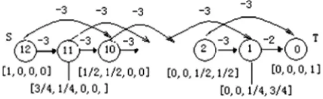
![Fig. 9. The 4-state problematic MDP [69].](https://thumb-ap.123doks.com/thumbv2/123dok/10905931.0/18.816.199.628.829.1013/fig-9-the-4-state-problematic-mdp-69.webp)