reproducing solar eruptions in the laboratory.

(1)

reproducing solar eruptions in the laboratory.

Thesis by

Quoc Bao N. Ha

In Partial Fulllment of the Requirements for the Degree of

Doctor of Philosophy

California Institute of Technology Pasadena, California

2016

(Defended June 16, 2015)

(2)

(3)

To my parents for their continual support.

(4)

Acknowledgments

I want to start by recognizing Paul Bellan, my adviser. My rst interaction with Paul was at a plasma physics conference in 2006. I was anxious about presenting my research at such a big conference. Paul was the rst person to stop at my poster.

He immediately put me at ease with a joke, and we clicked on a scientic, and on a personal level. I knew then that I wanted to go to Caltech to do research with him. The journey since that moment has been thoroughly enjoyable. I am amazed by how Paul sustains a high level of research output, while always making time for his students. He seems to have an endless capability to nurture the growth of his students. He is a great scientist, writer, and mentor. Above all, he is a generous human being, and I am truly blessed to have had the opportunity to grow under his guidance.

Thank you to my thesis committee members: Brent Fultz, Gregg Hallinan, and Jay Polk.

Brent Fultz chaired my candidacy committee. My interactions with Brent have been limited, but pleasant. I never felt rushed when meeting with him, and left those meetings relaxed and condent. Brent makes an eort to share the tasty snacks around his oce, and has a natural ability to connect with students. Thank you for guiding me from candidacy to defense.

It is dicult for students in the plasma group, to nd faculty members who can relate to our research. It was to my great surprise to learn that Gregg Hallinan researches coronal mass ejections on other stars. Gregg, I am very happy that you are on my committee.

My own interactions with Jay Polk have been pleasant, but I have also learned

(5)

a lot about Jay from others. While we were working on plasma physics problem sets, Angie Capece would occasionally mention how grateful she is to have Jay as an adviser. Rory Perkins mentioned that Jay asked some of the most insightful questions during Rory's defense. Jay, I look forward to sharing the bits that I have learned about space and plasma physics with you.

Thank you to the entire plasma group. Eve Stenson, Auna Moser, Deepak Kumar, and Rory Perkins are my senior. Of the four, Deepak is the most senior. Deepak's sense of humor, and his willingness to help the younger students stuck me. Auna and Rory stepped up after Deepak graduated. Both did admirable jobs of leading the way, and knowing what was going on. Rory is a close friend and mentor. I'm grateful for the time that he takes from his busy schedule to call me, and make sure that I'm doing OK. Thanks, man.

The most inuential senior grad student to my Caltech experience is Eve Stenson.

She shared an oce with me and was my mentor while she was here at Caltech. Eve is an excellent writer and thorough scientist. She is an excellent source of laboratory knowledge. I swiveled my chair around countless times to ask her questions, but she never seems to get sick of me. Thank you Eve!

Mark Kendall and I started graduate school together. We fed o each others jokes and I loved hearing the Mark's ridiculous stories. He is an excellent scientist and hilarious friend. Mark, I wish you all the best.

Xiang Zhai and Vernon Chaplin joined the group a little after I did, though we three are nishing at the same. Vernon is funny, disciplined, and an excellent scientist.

I'm grateful to both Vernon and his wife, Cathy Chaplin, for their friendship, and their tasty food. Vernon is instrumental in my post-graduation employment. Xiang is my scientist role model. He is funny, productive, and does not hesitate to help others with their work. His extraordinary accomplishments are matched by his authentic sense of modesty, making him a pleasure to work with.

Zachary Tobin joined the group a few years after I did. In research and outside of research, Zach is the guy who does what needs to get done. I'm grateful to Zach for wrestling with the IDL code to get the data acquisition system online.

(6)

Magnus Haw is an exceptional dancer, activist, and scientist. As his senior, I'm supposed to mentor him, to temper his expectations about experimental research, and to encourage his personal growth. Instead, I become a better scientist just by interacting with him. His programming skills, his work ethic, and his scientic intuition are top notch. Most importantly, he reminds me to take the time to ask to better questions instead of blindly solving poorly-posed questions. I have a little voice in my head that reminds me: what would Magnus do?

Thank you KB Chai for showing me how to be a productive scientist. The acknowledgments of previous graduate students gush about the benet of having a post-doc present to model the habits of a successful young scientist. It has been instructive to learn how you approach a challenging experimental task, and how you systematically derive its solution.

To the new grad students, Pakorn Wonwaitayakornkul, Ryan Marshall, and Young Dae Yoon: you guys have to take classes and soak up as much knowledge as possible before the seniors in the group graduate. It is quite a tall order but it is clear to me that all three of you are motivated learners. Keep up the good work.

I want to thank the SURF students Federico Presutti and Patricio Arrangoiz. You guys made my work with Hall sensors a whole lot easier.

Thank you Connie Rodriguez. Eleonora Vorobie, and Christy Jenstad for your administrative support. I hear horror stories from group alumni about how much worse it can get. You three make the paperwork, and other organizational tasks so easy to complete.

Thank you Dave Felt for help with the electronics. You and Paul provide continuity across dierent generations of graduate students. Your design tips have saved me hours of troubleshooting.

A great big thank you to machinist Mike Gerfen. You are an excellent machinist and a cool person. May your future be lled with many remote control car races, and many snowboarding extravaganzas. Thank you to Joe Haggerty, Ali Kiani, and Brad over at GALCIT. You guys took care of the precise machining, so that I could focus on drawing pretty shapes on a computer screen.

(7)

I am grateful to the support sta (Regina, Jose, and others) who keep Watson immaculate. I have seen Watson restrooms devolve into a terrible mess, and shudder to think of what would happen without the sta's diligence.

Keeping in touch with old friends is incredibly dicult, but Igor Konsakhar is the exception. This tenacious guy refuses to be forgotten, and is my link to my teenage years. Thanks man.

I've had great new friendships with Tulasi Parashar, Henry Kozachkov, Max Cubil- los, Brian Standley, Himanshu Mishra, Angie Capece, Devvrath Khatri, Sidd Bikkan- navar, Tommy Nguyen, Matthew Kelly, Andy Lampersky, Scott Geraedts, David Brown, and so many others.

In particular, Henry and Andy were excellent roommates and added air to my life. Henry's command of the English language is so powerful that I would pay money to listen to his tirades. I'm also harnessing his editing skills for good, which is a euphemism for asking him to read this entire thesis! He is loyal to his friends and family, and is the rst person that I would call if I run out of gas while riding a motorcycle on the freeway. Thanks for bailing me out man! As for Andy, I will only say that he is Andy-guy, and that it has been fun.

There are certain people around whom friendships at Caltech are linked. One such person is Paula Popescu, who is a tireless and caring friend. She organizes themed parties and fun outings, and is a binding force for many physics and applied physics friends, including Itamar Yaakov, Brian Willett, Kevin Engel, Evan O'Connor, Dan Betea, Laura Book, Essie, Milevoje Lukic, and Kari Hodge.

The Caltech Ballroom Dance Club has been an essential part of my experience here at Caltech. I want to acknowledge the many friendships, including Neil Hale- lamien, Catherine Beni, Raj Kulkarni, Artemis Ailianou, Vivian Zhang, Connie Wang, Jennifer Walker, Sophianna Banholzer, Caitlin Scott, Jay Daigle, Tom Tyranowski, Eduardo Garcia, Raina Storer, Lydia Dennis, Jessie Rosenberg, Victoria Chernow, Megan and Robert Nix, and Wendy Li. In particular, I want to thank Neil Hale- lamien for being a trusted condant, and a dear friend. I also want to acknowledge Catherine Beni for being an exceptional individual in so many ways. Caltech is a

(8)

nexus for talented people, and Catherine is a model for the excellence that comes from hard work and incredible intellect. She also plays a mean game of Super Smash Brothers, and is a wonderful friend. To her, I say: MUD!

One of the many treasures at Caltech are the folks at the Caltech Y. I've had the pleasure of working with Alycen Chan, Liz Jackman, Athena Castro, Greg Fletcher, and Christopher Kealy. The Caltech Y keeps Caltech students sane by organizing volunteering opportunities, hiking expeditions, movie outings, nal exam decompres- sion, and so much more. They have made my time at Caltech enjoyable, and I see them doing the same for many other students.

I want to thank Tom Mannion for his role in my development as a leader and a chef. Tom, Denise Okamoto, and Lorrie Yamakazi ensure that students have a blast at Caltech.

I would like to acknowledge Susan Hackwood and everyone at the California Coun- cil of Science and Technology for their role in my growth as a leader. Susan invited me to join her for CCST meetings and introduced me to many established scientists and policy makers. A tremendous portion of my growth can be attributed to Susan's time and attention. She is my role model, and I hope to make the same impact on those that I meet, as Susan has done for me.

Another part of my growth came from pursuit of Aikido. I owe a deep gratitude to Tim Sullivan and Erik Henriksen for introducing me to this ne art. They have both poured countless hours into my practice. In particular, I wanted to thank Tim for his mentoring and his friendship. One of my darkest times in graduate school came after realizing that I had wasted two years due to a miscalculation. Tim helped me recover physical and mentally from despair. The quirky British humor is a tremendous plus!

To all my friends at Daiwa: Hideki and Tomoko Okuda, Michael Head, Tom Atherton, Crystal Siri, Birte Feld, Evon and Jane Hochstein, Rick, Florian Morino, Eric, and so many others. Your endless friendships and open arms were welcome sights whenever I trained at the dojo. I want to particularly thank the late Jack Arnold Sensei and the late Toma Rosenzweig. They are both great martial artists with gentle souls and warm hearts.

(9)

If I were to claim that I have a second family, it would be the Hurt family. I thank Nicole Bouley-Ford and Will Ford for introducing me to the Hurts. I cherish the discussions about leadership and management with Bill Hurt. Sally Hurt is kind, intelligent, and full of bright smiles. Bill and Sally embody many of the traits that I hold in high regard: modesty, generosity, kindness, and a deep love for the people around them. These traits extend to the rest of the Hurt family and I want to thank Bernadette Glenn, Douglas Murray, Mark Purnell, Kelly Purnell, and their many children, including Alex, Lydia, Kate, Kristen, Stephanie, Molly, Emmy. It has been wonderful to spend time with you all. I want to thank Bernadette for being an advocate and mentor. It is my great pleasure to connect Bassam Helou with the Hurt family. Bassam has done a wonderful job of integrating with the Hurt family, and I am condent that he will do well. Finally, I want to thank Vivian for her friendship and support. She has my back when I needed help and is a model nurse.

I've had the pleasure of being close to Jamie Garman for many years. We connected on a deep level, and a large part of my personal growth can be attributed to this intelligent, beautiful, and driven woman; she brings out my silliness and knows how to make me laugh, even under the most distressing of times. Perhaps her great- est contribution to my growth is that she taught me how to recognize my own needs, and to speak up for what I want. For that and so much more, she has my deepest gratitude.

Last but certainly not least, I would like to thank my family. Those in my family do not express our love verbally. Instead, my parents work tirelessly to support us; I can not believe that they raised a family on a graduate student salary! My parents demonstrate their love through their unwavering devotion and support, as well as a plethora of loving insults. Being called a monkey in my childhood was annoying, but I cherish such playful insults in adulthood. To my sister, for putting up with with me as an older brother, and for dealing with having similar names while growing up:

that was really confusing! You have grown so much, and are making a dierence in the world while I'm still chugging away as a student. I can always count on you to ercely defend your brothers and to tell hilarious stories. To my little brother, for

(10)

growing up to be a cool guy: the eleven years between us did not stop us from having close bond. I'm very glad that you are around to take care of our parents while I am in grad school. You are a reliable guy, and I know that I can count on you.

(11)

Abstract

Coronal mass ejections (CMEs) are dramatic eruptions of large, plasma structures from the Sun. These eruptions are important because they can harm astronauts, damage electrical infrastructure, and cause auroras. A mysterious feature of these eruptions is that plasma-lled solar ux tubes rst evolve slowly, but then suddenly erupt. One model, torus instability, predicts an explosive-like transition from slow expansion to fast acceleration, if the spatial decay of the ambient magnetic eld exceeds a threshold.

We create arched, plasma lled, magnetic ux ropes similar to CMEs. Small, independently-powered auxiliary coils placed inside the vacuum chamber produce magnetic elds above the decay threshold that are strong enough to act on the plasma.

When the strapping eld is not too strong and not too weak, expansion force build up while the ux rope is in the strapping eld region. When the ux rope moves to a critical height, the plasma accelerates quickly, corresponding to the observed slow-rise to fast-acceleration of most solar eruptions. This behavior is in agreement with the predictions of torus instability.

Historically, eruptions have been separated into gradual CMEs and impulsive CMEs, depending on the acceleration prole. Recent numerical studies question this separation. One study varies the strapping eld prole to produce gradual eruptions and impulsive eruptions, while another study varies the temporal prole of the voltage applied to the ux tube footpoints to produce the two eruption types. Our experiment reproduced these dierent eruptions by changing the strapping eld magnitude, and the temporal prole of the current trace. This suggests that the same physics underlies both types of CME and that the separation between impulsive and gradual

(12)

classes of eruption is articial.

(13)

List of Figures

1.1 (From Fig. 6 of Ref. [1]) False alarm due to failed prediction about geo-eetiveness of Jan 10 event by current NASA & NOAA models.

The NASA and NOAA predictions are of a serious solar storm whereas measurements (in green) show little geo-consequence. . . 4 1.2 Temperature vs density chart for plasmas. (From: Contemporary Physics

Education Project). . . 7 1.3 (a) Particles make circular cyclotron orbits about magnetic eld lines or

helical orbits along the magnetic eld lines. (b) A particle experiencing both a magnetic and electric eld will tend to drift in the direction of Eˆ ×Bˆ. This movement is independent of the particle charge. . . 9 1.4 Cartoons depicting reconnection. (a) Two eld lines come together and

interact a magnetic null point. (b) The corresponding change in eld topology is associated with a release of energy. (c) Bulk plasma ows Uin carry magnetic eld lines ows towards a magnetic null. (d) The compression of eld lines creates a thin current sheet (red) where reconnection occurs. Outward plasma ow Uout carries newly reconnected ux away from the reconnection site. . . 12 1.5 (a) Ref. [2] showed that a strong strapping eld can inhibit plasma

expansion. (b) Ref. [3] demonstrated the eruption of a solar-relevant plasma structure by injecting hot plasma into the footpoints. . . 17

(19)

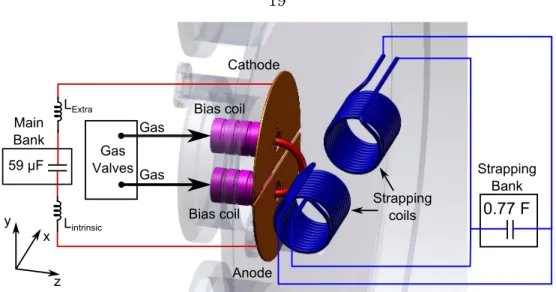
1.6 The cathode and anode dene the x−y plane of the coordinate system, with the gap separating cathode from anode dening the origin. The bias coils (purple) generate arched magnetic elds similar to a horseshoe magnet. Strapping coils (blue) are inside the vacuum chamber for the majority of the work in this thesis. . . 19 1.7 Application of cylindrical coordinate system to (a) a cylinder of radiusa

and lengthLand (b) a hoop of aspect ratioR₀/a. (c) A donut expressed in toroidal coordinates. . . 21 1.8 (a) CME with three part structure (from Ref. [4]) The front represents

density build-up in front of the CME, the so-called ux rope is the CME cavity, and the prominence is the core located at the bottom of the ux rope. (b) X-class are as viewed in 131 angtrom light. . . 23 2.1 Adapted from Ref. [5]. Paradigm with ares playing a central role.

Capital letters indicate observational phenomena and lowercase letters indicate physical processes or descriptive processes. . . 27 2.2 Adapted from Ref. [5]. Paradigm with CMEs playing a central role.

Capital letters indicate observational phenomena and lowercase letters indicate physical processes or descriptive processes. . . 28 2.3 Adapted from Ref. [6]. Over-simplied representation of pre-eruptive

conguration for sheared arcade models compared to ux-rope models.

The dark region represents the so called core eld where energy is built up. . . 31

(20)

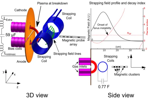
2.4 Schematic representation of experiment. The cathode and anode dene the x−y plane of the coordinate system, with the gap separating cathode from anode dening the origin. The bias coils (purple) generate arched magnetic elds similar to a horseshoe magnet. Independently powered coils (blue) produce strapping eld (green arrows) and the plot in the upper part of the side view shows how the strapping eld magnitude varies along the z axis. In the plot, the up-sloping dashed line (red) shows the calculated decay index of the strapping eld and the horizontal dotted line (red) shows the calculated instability threshold.

Additional inductance (L_extra) can be added to the intrinsic inductance of the system (L_intrinsic) to slow down the current pulse. The plasma (red) starts small but grows to many times its original size as it expands into the vacuum chamber. . . 33 2.5 Depiction of the hoop force. . . 35 2.6 Tension force comes from J_pol ×B_tor and is a consequence of the 1/R

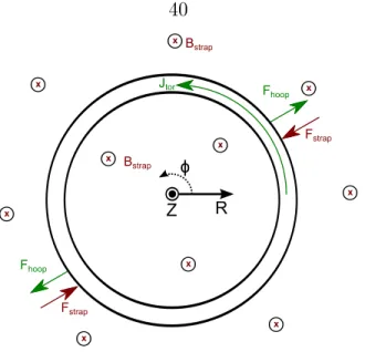
dependence of B_tor so that J×B₁ 6=J×B₂. The direction of the force is determined by J_pol, i.e., by whether the plasma is paramagnetic or diamagnetic. . . 38 2.7 Depiction of strapping force and hoop force. The strapping eld is ori-

ented into the page and interacts with J_tor. . . 40 2.8 Nearly-circular plasma connected to a black-box power supply. The

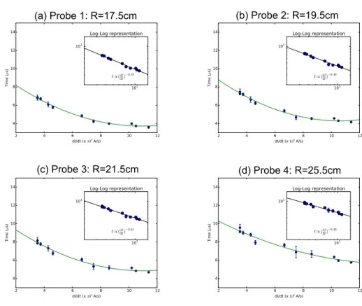
power supply can be (a) a short, (b) a voltage source, or (c) a current source. . . 42 2.9 Time for the plasma to travel to the magnetic probe clusters. dI/dtis

varied by changing the peak current I₀ and the rise time of the current pulse τ independently. The inset is a log-log representation of the data and shows the relation t_probe ∝(I₀/τ)^−γ where γ = 0.55,0.49,0.45, and

−0.39for probes 1-4, respectively. . . 49

(21)

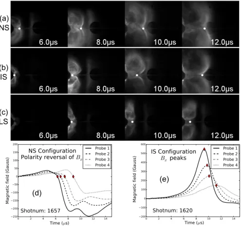
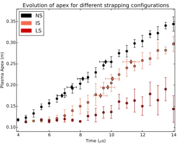
2.10 Imaging and magnetic diagnostics. The dots in (a), (b), and (c) represent the location of the plasma apex and are determined by looking at intensity slices along the z-axis and selecting the local intensity maximum. (d) and (e) show B_x component of the magnetic trace across all four magnetic probe clusters. The diamonds correspond to the bright (high density) leading edges from the camera images. . . 51 2.11 Height (z) vs time plot of dierent strapping congurations. The circles

represent data obtained from imaging the plasma. The diamonds represent plasma position determined by the magnetic probes. In the LS conguration, the plasma does not reach the magnetic probe in the 14 µs time interval. . . 52 2.12 (a) Velocity obtained by smoothing the distance vs time measurements

and then taking the numerical derivative for the three strapping congurations shown in Fig. 2.11. (b) Velocity as a function of apex height (z). (c) and (d) show acceleration obtained by smoothing the velocity and applying a numerical derivative. . . 53 2.13 (a) Measured voltage and (b) measured current for dierent strapping

eld congurations. (c) Calculated inductance vs time from voltage and current measurements using Eq. 2.25. . . 56 2.14 (a) Dierent current proles for the NS conguration. Blue represents

time before the plasma reaches the magnetic probe and green represents when the plasma is at the magnetic probes. (b) Average velocities before the magnetic probes (dark blue) and average velocities during the magnetic probe (dark green). The light green represents velocity just before the magnetic probes assuming the plasma starts in quasi-static equilibrium and experiences constant acceleration . . . 57

(22)

2.15 (a) Dierent current proles for the IS conguration. Blue represents time before the plasma reaches the magnetic probe and green represents when the plasma is at the magnetic probes. (b) Average velocities before the magnetic probes (dark blue) and average velocities during the magnetic probe (dark green). The light green represents velocity just before the magnetic probes assuming the plasma starts in quasi-static equilibrium and experiences constant acceleration . . . 58 B.1 Flux surface S moving with some velocityu⊥ with respect to the mag-

netic eld line. . . 98 B.2 Magnetic pressure and J×B for dierent congurations. . . 102 C.1 CSHKP phenomenological models for ares. . . 105 C.2 Adapted from Ref. [7]. This version is tailored to bipoles having sig-

moidally sheared and twisted core elds and accommodates conned explosions as well as ejective explosions. The rudiments of the eld conguration are shown before, during, and after the onset of an explosion that is unleashed by internal tether-cutting reconnection. The dashed curve is the photospheric neutral line, the dividing line between the two opposite-polarity domains of the bipoles magnetic roots. The ragged arc in the background is the chromospheric limb. The gray areas are bright patches or ribbons of are emission in the chromosphere at the feet of reconnected eld lines, eld lines that we would expect to see illumi- nated in SXT images. The diagonally lined feature above the neutral line in the top left panel is the lament of chromospheric temperature plasma that is often present in sheared core elds. . . 110

(23)

C.3 Cartoon demonstrating the basic concepts of ux cancellation. The initial eld (a) is sheared by ows along (b) and towards (c) the neutral line. This leads to reconnection in (d) and the submergence of lower loop CB. The overlying loops are also sheared (e) to eventually create the recognizable helical ux rope structure (f) and the ux line GF submerges. (from Ref. [8]). . . 112 C.4 Adapted from Ref. [9]. (a) Initial potential magnetic eld. The eld

is symmetric about the axis of rotation and the equator, so only one quadrant is shown. The photospheric boundary surface is indicated by the light gray grid. Magnetic eld lines are colored (red, green, or blue) according to their ux system. Two types of blue eld lines are indicated:

higher-lying light blue unsheared eld and low-lying dark blue eld that is sheared later in the simulation. (b) Force-free eld after a shear of π/8. The eld lines shown correspond to those in (a) and are traced from the same footpoint position on the photosphere as in (a). (c) As above, but for a shear of 3π/8. (d) As above, but for a shear of π/2. . 113 C.5 Adapted from Fig. 3 of Ref. [10]. Magnitude of equilibrium currentI vs

height for region NOAA 131 for whichh₁ = 1600km andh₂ = 12000km.

The arrows indicate the direction of the Lorentz force for a perturbation from equilibrium. A and B correspond to regions h < h₁ and h < h₂, respectively. C and D correspond to h > h₂. The Lorentz force due to interactions with the ambient eld dominates in regions A, B, and C where gravity dominates for regions D. . . 115

(24)

C.6 Adapted from Figs. 3-4 in Ref. [11]. The graph is a normalized equilibrium height h as a function of the reconnected ux φ for r = 10⁻⁵. As φ increases, the lament follows the lower branch of the equilibrium curve towards the critical point (lower equilibrium) atφ = 11.23. At the critical point, the equilibrium solution has an additional solution at the upper equilibrium and the plasma is expected to erupt upwards. The contours are the vector potential of the lament. The contour levels are not the same in all the plots though the relative location of the rising current channel is at the center of the concentric contour lines. . . 117 C.7 Adapted from Figs. 3 and 5 of Ref. [12] . . . 119 C.8 Adapted from Ref. [13]. A current channel of major radius R, minor

radiusa, footpoints separationS_f. The channel contains magnetic elds B_p and B_t. The subphotospheric eld is incoherent with B_p B_t. . . . 121 D.1 Representative side and end view of experimental set-up. . . 126 D.2 Scaled rendering of the Alpha and Bravo chambers compared to a 5-foot

human being. . . 127 D.3 Plasma breakdown process for (a) co-planar and (b) co-axial plasma

guns. (SSX coaxial cartoon adapted from Ref. [14]) . . . 128 D.4 (a) Simulation of horse-shoe shaped eld-lines generated by the red and

blue bias coils. Darker color lines represent eld line that are closer to the axis of the coils. (b) Cooke camera image of left-handed (reverse-S) sigmoid. The current ows from bottom foot-point to top foot-point and is anti-parallel to the bias eld. (c) The bias eld goes from the top (red) coil to the bottom (blue) coil, creating a reverse S sigmoid. (d) The bias eld goes from the bottom (red) to the top coil (blue) creating a right-handed sigmoid (S shape). . . 130 D.5 Evolution of the electrodes over the thesis work. The blue and red parts

represent the polarity of the bias coils used to construct horse-shoe- shaped magnetic elds. . . 131

(25)

D.6 (a) Simple construction of the coil. (b) Picture demonstrating how the coil is mounted on the plasma gun. The coils in the image are adjusted to be in the Large conguration. (c) Representation of the plasma discharge circuitry. The system capacitance and resistance areC andR, respectively. The total system inductance can be changed by adding an adjustableL_extra. (d) The current prole for dierent coil congurations when the plasma bank is charge to 3 kV. . . 133 D.7 Geometry of single plasma loop and Ref. [15] representation of eight

spider legs. . . 135 D.8 (a) Variation in the current prole for dierent strapping elds when

L_extra = 0 nH. (b) when L_extra = 370 nH. Shaded region represents shot-to-shot variations. . . 136 D.9 Strapping eld lines (green) produced by (blue) coils (a) in bipole con-

guration (b) in coaxial conguration. . . 137 D.10 Overview of dierent coil congurations. (a) and (b) are outside the

vacuum chamber, behind the plasma gun. (c) is inside the vacuum chamber in front of the plasma gun. . . 139 D.11 Welding cable coils are large and placed a distanceh₀ behind the plane

of the electrodes. . . 140 D.12 (a) Magnetic forces on coil when pulsed with current. (b) Coil mounted

on Delrin support structure. (c) Photo of coil. . . 141

(26)

D.13 (a) Custom support structure for Encore coils. The structure is designed to not have closed conductive loops. (b) Two G-10 sheets sandwich the coils. Regularly spaced holes on the sheet allow discrete displacement.

(c) Linear slides permit ne adjustments of coil position. (d) MDC ange with two 1/4 copper tubing for current input and output. The tubing is hollow and the system designed so that a cooling medium be injected into the pipes. (e) Schematic view of plasma coil support structure.

Adjustable carriages can be mounted to dierent holes on the support structure allowing exible placement of the coils. (f) End-view photo of strapping coils set-up. . . 143 D.14 Typical position of Imacon and Cooke cameras viewed from above the

experiment. The plasma, strapping coils, electrodes, and bias coils are shown in red, blue, orange, and purple, respectively. . . 144 D.15 (Adapted from Refs. [16] and [17]) (a) Commercial inductors placed are

placed in retention xture allow high spatial resolution. (b) Image of solar magnetic probe. . . 146 D.16 (a) A comparison of the signals measured by the isolated high voltage

probe and the Tektronix high voltage probe. Each signal represents average of about 10 shots. (b) Comparing voltage and current trace.

The voltage probe indicates bursts of noise (dashed blue circles) when the current trace ips polarity and or has a disruptive spike.. . . 148 D.17 Rogowski coil with a built in passive integrator. This particular con-

guration is eective at measuring current at high frequencies where i₂R V_cap but not so high so that i₂R Ldi₂/dt, where L is the inductance of the Rogowski coil. . . 150 E.1 Hall eect when the magnetic eld is perpendicular to the sensor. . . . 153

(27)

E.2 The hall sensor control circuit has three parts: current mirror, hall elements, and amplication circuitry. A current mirror is used to provide the same amount of current to each hall element and the dierential output is processed by the instrument ampliers . . . 156 E.3 The current passing through the transistor Q1 is theoretically mirrored

through transistors Q3, Q4, and Q5. The amplitude of this current is determined by the value of V_dd and R1. Transistor Q2 prevents the circuit from saturating if one of the loads (U1, U2, U3) fail. . . 157 E.4 PCB representation of circuitry in Figure E.2. Both the control circuitry

and the surface mounts for two 3-axis sensors are printed in the same board. The boards are cut along the dotted red lines. Hall elements are placed on the footpoints marked by the purple circle and the components enclosed in blue are assembled and placed perpendicular to one another like in Fig. E.5 (a). . . 159 E.5 (a) 3-axis hall sensor element made by placing PCB pieces perpendic-

ular to each other. A polycarbonate angle supports the plates. (b) An exploded view of a hall sensor mounted on a carriage. The sensors are surrounded by a polycarbonate shell lled with RTV silicone. (c) Six sensors are mounted on a board. The entire set-up is mounted on the vacuum chamber ports. (d) Photo of set-up. The blue and white Eth- ernet cables bring current to and carry the output signals from the hall sensors. . . 160 E.6 (a) Set-up with placement of welding cable strapping coils, quad

plasma gun, and Hall probe. (b) Measured magnetic eld from hall sensors. (c) Simulated magnetic eld. . . 163 E.7 (a) Set-up highlight the activated bias coils and hall probe. (b) Measure-

ment of magnetic eld due to bias coils (c) Measurement of magnetic eld including . . . 164 E.8 Visualization of magnetic eld in region above strapping coils. Magnetic

eld strength is in Teslas. . . 165

(28)

E.9 (a) Support structure for Hall sensors near the electrodes. The set-up permits the adjustments of Hall sensor placement along all three di- rections. (b) Measured bias eld along a single plane. (c) Measured strapping eld along a plane. (d) Magnetic measurements of both bias and strapping eld. . . 166 E.10 (a) Peak magnetic eld not a linear function of voltage. (b) The prole

of the magnetic eld pulse varies with diering bias bank voltage. (c) Bias magnetic eld prole diers from measured bias coil current. . . . 167 F.1 Set-up for calculating the magnetic eld for a loop of radius a with

current I. . . 170 F.2 Phi and theta rotation are rotations about the y and z axis, respectively. 170 F.3 Darker lines represent eld lines which originate closer to the center of

the coil. . . 171 F.4 Field line trace for superposition of bias eld from purple coils with

varying strapping eld from blue coils. Green/red represent eld lines from the bias/strapping coils, respectively. Darker eld lines are closer to the axis of their source loop. . . 172 G.1 Representations of normal (solid) vs stereographic (dashed) projections.

The same point of displacement H at a distance D maps into ρ < r, thus allowing the stereographic projection to have a wider eld of view. 175 G.2 Uncorrected image (left) and corrected image (right). The corners show

the most noticeable change. The corrected image has also been cropped so that the nal image has the same number of pixels. The resampling can sometimes introduce artifacts like the small white dot in the oppos- ing port (large black circle in center of image). . . 175 G.3 Percentage error on Nikon CCD from using the sheye lens. The dotted

square represents the much smaller Imacon CCD, for which the distor- tion is limited to 20% near the corners. . . 177

(29)

G.4 (a) Automatic circle nding algorithm fails to locate the port but nds many false positives. (b) A least squares t easily captures the port from three user clicks. . . 178 G.5 Set-up as viewed from top of chamber. Since L d, a small θ may

result in Lsinθ ≈d. . . 178 G.6 (a) Method of determining a rotation θ about the y axis. Here,f is the

focal length of the lens and ∆x₁ and ∆x₂ are the displacement of the objects on the image. b is the distance along the zˆ direction between the port and the coil center while b+x is the distance from the coil to the camera. In general, black lines correspond to measurements in the unrotated system and blue lines correspond to quantities in the rotated system. (b) The same technique applied to rotations about the z axis. 180 G.7 Plasma apex tracking program. . . 182 G.8 Schematic with typical magnetic probe placement relative to the plasma

gun. . . 183 G.9 (a) Typical magnetic traces showing all three component of the mag-

netic eld. The magnetic trace changes dramatically ((b) and (c)) when strapping eld is applied. . . 184 G.10 Measurement of the B_x component of the magnetic eld across all four

probe clusters. (a) The B_x component switches signs when the plasma passes the probe and provides velocity information about the plasma.

(b) When a strong strapping eld is applied, the magnetic ux is frozen and carried by the dense region of the plasma. One should employ the peak of the B_x instead of the zero-crossing, . . . 185 G.11 (a) Three component magnetic traces comparing left and right handed

plasmas. (b) Cooke camera end-on imaging of reverse-S left-handed plasma. . . 185 G.12 (a) Polarity reversal ofB_x used for qualitatively dierent congurations.

(b) This technique can give good measurements provided that the feature being tracked persists across probe clusters. . . 186

(30)

G.13 Current prole while (a) varying the bias bank voltages, and (b) varying the gas power supply voltages. . . 187 G.14 (a) Current prole while varying strapping eld. (b) Normalized peak

current while varying the strapping bank voltage. . . 189 G.15 Schematics of coaxial railgun. A conductive spheromak propagates down

a coaxial guide representing an LC circuit with increasingL. . . 190 G.16 Comparison between a basic simulation of current as a function of time

and the measured current. . . 192 G.17 Compare simulation to data when resistance is taken into account . . . 195 G.18 (a) Varying L_i and R to obtain best t to current trace in Maximum

L_extra conguration, (b) Measured L_extra compared to estimate from t. 197 G.19 (a) Measured current in 'Maximum' conguration compared to model

ts with two/three free parameters. (b) Calculated nominal system inductance from model . . . 198 G.20 Fitting current trace prole associated with two dierent strapping bank

voltages (0 V and 90 V), by adjusting free parameters: (a) Q, (b), l⁰, (c) L, (d) R. . . 199 G.21 Best tted main bank voltage as function of strapping bank voltage. . 200

(31)

List of Tables

2.1 (Reproduction) Energy requirements for a moderately large CME . . . 29 2.2 (Reproduction) Estimate of Coronal Energy Sources . . . 29 D.1 Measured value of the inductance . . . 134 D.2 Parameters of strapping coils used . . . 138 E.1 (Reproduced from from Table 1.1 of Ref. [18]) Intrinsic carrier concen-

tration at 300^oK . . . 155 G.1 Dimensionless parameters. . . 192 G.2 Parameters obtained from Ref. [15] . . . 192

(32)

Chapter 1 Introduction

1.1 Thesis outline

This thesis is written for two separate audiences: (i) thesis committee members who are presumed to be interested in the results and (ii) future graduate students, who are presumed to be interested in the details. As such, the thesis main body attempts to be succinct with only the relevant details, whereas the appendix is lengthy. The reader is encouraged to peruse the appendix to view useful denitions, mathematical relationships, nuts and bolts, and an in-depth look at some of the solar models. Due to the organization of this thesis, there will be some repetition between the main body and the appendix.

The basic structure of the thesis is as follows. The introduction motivates the study of the sun, presents a brief introduction to plasma, describes the experimental setup, and denes important solar terminology. Chapter 2 is dedicated to the reproduction of the slow rise to fast acceleration of a solar eruption. This chapter contains an overview of the debate, the set-up, a generalized implementation of torus instability, results, and discussions addressing important questions in solar physics.

Chapter 3 gives the conclusion. The conscious decision to have a single main chapter is due to the time restrictions for thesis writing.

(33)

1.2 The sun

It is dicult to exaggerate the importance of the Sun to life on Earth. Evidence of the prime role of the Sun is evident in its status as a deity among human civilizations and cultures¹. With the power to sustain life comes the power to harm, and the sun is certainly capable of violence. Large solar eruptions release energetic particles and magnetic energy into the solar system. If these eruptions hit the Earth, the solar magnetic eld can cancel out part of the Earth's magnetosphere, eectively lowering the Earth's protective shields and resulting in powerful geomagnetic storms.

Countless solar eruptions have impacted the earth since the beginnings of civiliza- tion, but societies are increasingly susceptible to geomagnetic storms, since modern humans depend on an always-functioning electrical infrastructure. In 1989, a solar eruption caused a geomagnetic storm which induced large electric currents in the long-distance electrical power transmission lines in Quebec, Canada. These currents interacted with and overwhelmed transformers, causing catastrophic failures, and the entire province was left without electricity for over nine hours! Another example is the outage of two Canadian telecommunications satellites in January 1994 due to enhanced energetic electron uxes. Even though the rst satellite recovered after a few hours, the repair of the second satellite took 6 months and costs over 50 million dollars [19].

A recent near miss event occurred in July 2012 when a coronal mass ejection (CME) hit NASA's Solar Terrestrial Relations Observatory (STEREO [20])-A, a satellite on the same solar orbit as the Earth but during the eruption was located ahead of the earth by about a week [21]. Scientists used STEREO-A's magnetic measurement to model the theoretical impact of this CME had it struck the Earth. Their models predicted a larger storm than the 1989 Quebec storm in the best case scenario and a storm surpassing the largest solar storm on written record in the worst case scenario.

This largest solar storm is known as the Carrington event of 1859 and was reported to have caused auroras as far south as Hawaii, and to have knocked out the global

1Solar gods include the Aztec Huitzlopochtli, the Mayan Kinich Ahau, the Egyptions Ra, the Greek Helios, the Roman Sol, the Arabian Malakbel, etc.

(34)

telegraph network.

The close-call of July 2012 motivated question about the frequency of extreme solar storms and the likelihood of Earth impact. Riley [22] assumed that the frequency of occurrence scales as an inverse power of the severity² and estimated the probability that another Carrington-like storm would occur in the next decade to be 12%. This is comparable to the likelihood of a serious earthquake in California over the same time interval. A 2008 National Academy report [19] estimates the cost of a severe geomagnetic storm scenario to be 1-2 trillion dollars, with a recovery time of 4-10 years.

One major dierence between solar storms and earthquakes is that scientists can obtain early warning from satellites observing the sun and potentially predict oncom- ing solar storms. Unfortunately, predictions of solar eruptions are exceedingly dicult and the arrival times of signicant space weather events have only been accurate to

±12 hours [20]. Much of the uncertainty is due to the complicated nature of eruptions. After leaving the solar atmosphere, erupted structures can confound simple estimates by speeding up, slowing down, or rotating. The ambient solar eld may deect the eruption, resulting in non-radial propagation [23]. Many models do not consider these nuances and instead rely on nominal values to make their predictions.

The community has not agreed on the geometry of the eruptive structure, resulting in a healthy debate between 2-D loops, spherical shells, cylindrical shells, ice-cream cones, and graduated cylindrical shells (side view of arched structure) [4, 24].

The magnetic eld orientation also plays a central role in how solar eruptions interact with the earth. CMEs with a southward magnetic eld can cancel the Earth's northward magnetic eld, thereby enhancing the injection of magnetic energy into the Earth's magnetosphere. In contrast, northward-directed solar magnetic elds have minimal interactions with the Earth [25]. Even though the magnetic orientation of the eruption determines whether a storm will have a catastrophic impact, most existing space weather models do not include information about the underlying magnetic structure [26, 27]. These models rely on measurements from spacecraft at the

2This is similar to the scaling of earthquake frequency and their severity.

(35)

Figure 1.1: (From Fig. 6 of Ref. [1]) False alarm due to failed prediction about geo-eetiveness of Jan 10 event by current NASA & NOAA models. The NASA and NOAA predictions are of a serious solar storm whereas measurements (in green) show little geo-consequence.

rst Lagrangian position to determine the magnetic orientation. This means that information about the magnetic eld orientation is not available until approximately 1 hour before Earth impact. Unfortunately, this may not be enough time to arrive at the correct prediction.

There are societal consequences for accurately predicting low-probability high- damage events, as demonstrated by the L'Aquila, Italy earthquake and corresponding debate [28]. The trials of the Italian scientists who failed to predict this earthquake highlight the challenges of communicating probabilistic events to the general community. Scientist must balance a 98 percent probability of a false alarm against a 2 percent chance of failing to issue a warning for a catastrophe. While the L'Aquila event focused on the latter, there are tangible consequences associated with false alarms. One example of a solar eruption false alarm is from Ref. [1] and shown in Fig. 1.1. Scientists use a logarithmic Kp index to predict the severity of a solar event whereKp≥5is considered a solar storm and Kp= 8 represents a severe solar storm. The latest NASA and NOAA models predicted a powerful storm but actual Kpmeasurements shown in green reveal negligible consequences due to the eruption.

There is much to be done in order to improve our space weather predictive ca- pabilities. In theory, we should be able to predict an upcoming solar storm through accurate modeling of the underlying physics. Unfortunately, there is no standard

(36)

model for CMEs and much of our understanding is still empirical and based on qualitative arguments about magnetic eld lines.

1.3 Motivating questions

There are many hotly debated solar physics questions as of the writing of this thesis [29] and two of these will be addressed herein. The rst question is most fundamental:

what causes the slow-rise to fast eruption of CMEs? The next question is 'Should fast and slow CMEs be attributed to dierent models?' In the process of addressing these questions, we create a framework that unies two dierent models of solar eruption.

1.3.1 Demonstration of slow-rise to fast eruption.

Measurements of CMEs near the earth are consistent with coherent magnetic, twist- carrying coronal structures (i.e., ux ropes) [4, 30], but there is debate on whether the ux rope structure existed prior to the eruption or if it was formed during the eruption by magnetic reconnection. Recent observations [31] and simulations [32]

suggest that the magnetic ux rope structure exists before the eruption and triggers the eruption through a loss of equilibrium mechanism. One such mechanism, the torus instability [33], occurs when a strapping eld in the corona decays sharply as a function of height, allowing a rapid acceleration of the ux rope when it rises above a critical height.

We reproduce the slow rise to fast acceleration of laboratory ux ropes in the lab, and our results are in agreement with the torus instability.

1.3.2 Impulsive vs Gradual CMEs.

Historically, CMEs are divided into two categories: impulsive (fast) and gradual (slow) [29, 34]. Impulsive eruptions occur at very high speeds and decelerate while gradual CMEs exhibit a slow acceleration³. It is thought that impulsive CMEs are tied to

3Impulsive CMEs velocities are over 750 km/s whereas gradual CMEs velocities are around 400 km/s.

(37)

are-associated events while gradual CMEs are associated with lament eruptions.

There is recent evidence, however, that such a distinction may be articial. Feynman and Ruzmaikin [35] present observations of a fast, are-associated CME with corresponding erupting lament. Statistical studies by Vrsnak et al. [36] and Yurchyshen et al. [37] found no reason to separate the two types of CMEs. Chen & Krall [38]

and Torok & Kliem [39] numerically reproduce impulse and gradual CMEs by ux injection and by torus instability, respectively.

We are able to produce impulsive and gradual CMEs in the laboratory by changing the prole of the current trace (ux injection), and by changing the strapping eld (torus instability). We expect the sun to use both approaches to produce fast and slow CMEs, so the distinction between impulsive and gradual CMEs is likely articial.

1.3.3 Unifying ux injection and torus instability

The Kliem & Torok implementation of torus instability [33] focuses on the prole of the strapping eld interacting with a current loop. The ux injection model [40]

focuses on the applied voltage across the footpoints of a plasma arch. Chen [41] argues that the Kliem & Torok implementation does not have footpoints, and is therefore inconsistent with the boundary conditions. Our experiment has footpoints, adjustable strapping eld proles, and adjustable voltage proles, so elements from both models are applicable.

We present a simple model for a nearly-circular plasma, with boundary conditions determined by an adjustable power supply. This model connects ux injection and torus instability to our experimental setup.

1.4 Introduction to plasmas

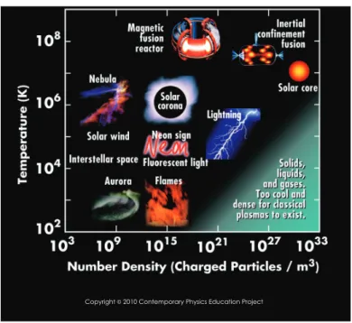
Plasmas are ionized gases and make up 99 percent of the known universe. However, the typical human environment is too dense and too cool for plasma to exist. Figure 1.2 is a log-log plot of temperature and density; solids, liquids, and gases occupy the lower right hand corner of the plot whereas plasma makes up the rest of the gure.

(38)

Figure 1.2: Temperature vs density chart for plasmas. (From: Contemporary Physics Education Project).

Plasmas can be cool and diuse like the beautiful auroras of the polar skies or dense and extremely hot like the center of the sun. Their ionized nature means that their behavior is inuenced by magnetic elds. The three fundamental parameters that characterize a plasma are: temperature, number density, and magnetic eld [42].

Consider plasmas with equal numbers of positive and negative charges⁴. Even though the plasma is considered neutral as a whole, there are localized regions of strong electric eld. Within these regions, the forces due to an isothermal pressure gradient must balance the electrostatic electric eld to determine the localized density distribution. Assuming that thermally induced perturbations are sucient slow, the density distribution of the electrons and ions are given by the Boltzmann relation

n_σ =n_σ,0exp(−q_σφ/κT_σ)

where σ ∈ {e, i} is the particle species, T_σ is the temperature, q_σ is the charge, φ is the electrical potential, κ is Boltzmann's constant, and n_σ,0 represents a constant

4Non-neutral plasmas contain only a single charge and dusty plasmas also include charged dust as a third type of particle.

(39)

density.

The charges self-organize because same-polarity charges repel and opposite-polarity charges attract; this self-organization creates an eective screening eect. For example, an ion will attract electrons around it while repelling nearby ions. The charge of the surrounding electrons screen the charge of the ion so that an observer suciently far away will not see the electric potential associated with the ion. The length scale of this screening eect plays a fundamental role in plasma physics and is known as the Debye length:

λ_D ≈λ_D,e =

₀κT_e ne²

1/2

wheren≈n_iis the system density and the system Debye length (λ_D) is approximately the Debye length of the electrons(λD,e). This self-organization occurs for all particles in the plasma and only makes sense if enough particles exist within a volume (λ³_D) to provide screening. Thus, a criterion for an ionized gas to be considered a plasma is nλ³_D 1, where n is the number density of the ionized gas [42]. In order for the shielding to be relevant, the plasma characteristic length must be much greater than the Debye length so that the plasma can be considered quasi-neutral. Thus, the two dening features of a plasma are:

1. nλ³_D 1 2. Lλ_D

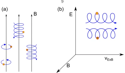
The inclusion of a steady state magnetic eld introduces interesting behavior to individual particles and to the collective plasma. A charged particle in a magnetic eld exhibits cyclotron motion by making circular or helical orbits along a guiding center as shown in Fig. 1.3 (a). If both electric and magnetic elds are present, the particle undergoes an E×B drift as shown in 1.3 (b). This drift is independent of the charge of the particle, so both positive and negative charges move in the same direction. Things get even more interesting when the particles follow curved magnetic eld lines or enter a non-uniform and/or time dependent magnetic region. Needless to say, plasmas exhibit many complicated but interesting behaviors; the eld of plasma

(40)

B

+

E

-

B

v

_ExB

(a) (b)

-

Figure 1.3: (a) Particles make circular cyclotron orbits about magnetic eld lines or helical orbits along the magnetic eld lines. (b) A particle experiencing both a magnetic and electric eld will tend to drift in the direction ofEˆ×Bˆ. This movement is independent of the particle charge.

physics attempts to describe the essential concepts behind these behavior.

1.5 Magnetohydrodynamics

There are many levels of plasma description from tracking individual particles to magnetohydrodynamics (MHD); additional information about the dierent description of the plasma can be found in Sec. B.1. MHD approximates the plasma as a single conductive uid and is the least accurate of all the descriptions. Nevertheless, it is still tremendously useful because many systems do not require the additional precision of the other descriptions and MHD provides the most ecient and intuitive method for assessing the plasma. Complicated geometries are also dicult to model and are often only analytically feasible in the context of MHD.

The MHD equations relevant to solar phenomena are:

• The continuity equation:

∂ρ_m

∂t +∇ ·(ρ_mU) = 0 (1.1)

(41)

where ρ_m is the mass density andU is the center of mass velocity.

• The equation of motion:

ρ_mDU

Dt =J×B− ∇P −ρ_mg (1.2)

whereJis the current density,Bis the magnetic eld,P is the thermal pressure, and ρ_mg is the force of gravity, which is typically important on the Sun but is not found in standard MHD derivations.

• Ohm's law for resistive MHD:

E+U×B =ηJ (1.3)

where E is the electric eld andη is the plasma resistivity.

• Faraday's law:

∇ ×E=−∂B

∂t

• Ampere's law in the limit of velocities much less than the speed of light:

∇ ×B =µ0J

• Divergence free condition:

∇ ·B= 0

• Energy equation of state:

P ρ^5/3m

=const (1.4)

where γ = 5/3 for an adiabatic equation of state.

MHD focuses on low-frequency, long-wavelength, and magnetic behavior of the plasma.

The following conditions are required for MHD to be valid:

(42)

• Quasi-neutrality, meaning that the characteristic length scale must be much larger than the Debye length (λ_D).

• The plasma must be collisional. This means that collision time is much less than the time scales of interest so that the pressure can be approximated as isotropic and the system is at a near Maxwellian.

• Characteristic velocity is much slower than the speed of light, meaning that the displacement term is dropped from Ampere's law.

• Characteristic time scale of phenomena is long compared to electron cyclotron motionqB/m so that the electron inertia term can be dropped.

In the limit when resistance is negligible (η →0), the system is known as Ideal MHD.

The concept of frozen-in ux (Sec. B.2) is important in ideal MHD. It is intuitive to think of frozen-in ux as plasma and magnetic eld lines moving as an ensemble in order to preserve the eld-line topology [42]. This is a strong topological constraint which prevents the magnetic eld lines from tearing and reconnecting even if doing so would result in an energetically favorable conguration. Thus, even a small amount of resistivity can have large impacts on plasma stability since it allows the plasma eld line topology to change within localized regions.

1.6 Magnetic Reconnection

Magnetic reconnection describes the topological change of a magnetic conguration due to a tearing and reconnecting of magnetic eld lines at a magnetic null point (Fig. 1.4 (a)). The resulting change in the topology allows the system to relax to lower energy congurations, thereby releasing free energy (Fig. 1.4 (b)). This free energy has been attributed to many space processes, including the Earth's magnetosphere, solar ares, and star formation [29, 43, 44]. Reconnection has also been observed in laboratory experiments [4547].

The simplest reconnection model is the Sweet-Parker reconnection [48, 49]. Flows of plasma bring magnetic eld lines together so that eld gradients become strong at

(43)

L

x δ x

y U_in

U_in U_in

U_in

U_out U_out

(c) (d)

(a) (b)

Magnetic null point

Free energy release

Figure 1.4: Cartoons depicting reconnection. (a) Two eld lines come together and interact a magnetic null point. (b) The corresponding change in eld topology is associated with a release of energy. (c) Bulk plasma ows U_in carry magnetic eld lines ows towards a magnetic null. (d) The compression of eld lines creates a thin current sheet (red) where reconnection occurs. Outward plasma ow U_out carries newly reconnected ux away from the reconnection site.

(44)

a localized region (Fig. 1.4 (c)). The interaction of eld lines forms a thin current sheet (Fig. 1.4 (d)) where non-ideal MHD reconnection behavior occurs. The rate of reconnection is determined by the dimensions of the current sheet (δ,L), which scale as:

δ

L = 1

√Sin

(1.5) whereS_inis the inow region's Lundquist number. The Lundquist number, a measure of how well the magnetic eld is frozen into the plasma, is

S_in = µ₀v_a,inL η

where va,in =Bin/√

µ0ρm is the Alfven velocity of the inow, and η is the resistivity of the system.

While a general Sweet-Parker reconnection model has been demonstrated in the laboratory [50], the reconnection rate predicted by Eq. 1.5 is many orders of magnitude too slow to describe solar ares [51], which have Sin ∼ 10¹¹. This slowness in Sweet-Parker is attributed to the pile-up of the large amount of mass that must ow through the very narrow (∼δ) current channel. Petschek [52] proposed that, outside the immediate reconnection region, standing waves could drive outows, dramatically increasing the reconnection rate. The Petschek model predicts reconnections rates that scale as

vout

v_a ∼ 1 ln(S_in)

which is insensitive toS_in. Nevertheless, the Petschek model has been criticized as not being self-consistent [53] and modern researchers are looking beyond Resistive MHD towards the smaller length scales when ions are no longer considered magnetized [5456]. This regime Hall MHD reconnection is a current topic of research and the details can be found in Ref. [43].

(45)

1.7 Dimensionless form

A remarkable feature of plasmas is that the same qualitative phenomena occur in plasmas with temperatures, densities, and magnetic elds that dier by many orders of magnitude. This scalability permits predictions about novel behavior using intuition about known plasma behavior. One way to take advantage of the scalability of plasmas is by rewriting the MHD equations in dimensionless form to extract dimensionless constants. In particular, the continuity equation (Eq. 1.1) and the equation of motion (Eq. 1.2) become

∂ρ¯_m

∂τ¯ =−∇ ·¯ ( ¯ρ_mU)¯

¯ ρ_m

∂

∂τ¯ + ¯U·∇¯

U¯ = ∇ ×¯ B¯

×B¯ −β∇¯P¯+γρ¯_mg¯ (1.6) and the induction equation is obtained by taking the curl of resistive Ohm's law (Eq.

1.3), yielding

∂B¯

∂τ¯ =∇ ×( ¯U×B) +¯ 1 S

∇¯²B¯ (1.7)

Three dimensionless constants capture the essential physics of the system:

β = 2µ₀P

B² (1.8)

S = µ₀Lv_A

η (1.9)

γ = gL

vA (1.10)

where L is a typical length scale and v_A = B/√

µ₀ρ_m is the characteristic Alfven velocity. The plasma β is a ratio of thermal pressure to magnetic pressure. The Lundquist numberS is a ratio of Alfven time scale to the resistive time scale. There is no standard name for γ which compares the gravity to magnetic forces.

In the solar corona, andβ 1so magnetic forces dominate thermal forces. S1, which means that the plasmas are highly conducting and Ideal MHD is applicable.

The magnetic energy density is 800 times more powerful than the gravitational energy density in the solar corona [57] so γ is negligible.

(46)

1.8 Limits of observation and numerical studies

Observation of solar laments, arched plasma structures associated with eruptions, have various limitations. Solar observations are unable to measure the magnetic eld in the corona precisely and so solar models extrapolate the coronal magnetic eld from photospheric magnetic measurements [32, 58]. The best photospheric magnetic measurements are obtained from laments positioned on the face of the sun, but observers lack the ability to determine the geometry and conguration of those laments directly; the converse is true for laments close to the limb of the sun [59]. As a result, eruptions with excellent imaging diagnostics are severely lacking in magnetic information. Even when quality photospheric magnetic measurements are available, the process of extrapolating the magnetic eld into the corona has its limitations.

Extrapolation results dier depending on the underlying assumptions [30] and even the best non-linear force-free algorithms struggle to extrapolate the force-free corona magnetic eld from the boundary measurements obtained from a forced photosphere [60].

The methods of modeling the magnetic eld listed in increasing levels of sophisti- cation are potential eld source surface, force-free eld, non-linear force-free eld (NLFFF) employing line-of-sight magnetograms, NLFFF employ complete vector magnetograms, and MHD models. The advantage of the eld models is that they are data-driven and constrained by observations. Unfortunately they are static, so independent eld models must be generated for each time step to evolve the system. In contrast, MHD models are intrinsically dynamic but they are initialized by idealized magnetic elds and are not constrained by observations. Almost all solar eruptions models suer from poor knowledge about the initial conditions of the magnetic eld and this problem is unlikely to be addressed until satellites are sent to directly probe the sun⁵.

Although we have more satellites in the sky than ever before, there are limitations to what can be done observationally. Scientists do not have control over the behavior

5See: Solar Probe Plus mission set for 2018 launch.

(47)

of the Sun and must wait for it to do something interesting. The sun is happy to oblige with powerful eruptions during solar maximum but can also stubbornly refuse to display interesting eruptions during periods of solar minimum. When an eruption occurs, scientists hope that satellites are properly positioned to image the event. Most satellites are along the Sun-earth axis and thus provide a single view of eruptions. A pair of satellites (STEREO-A and STEREO-B [20]) y ahead and behind the earth and the additional perspective of an eruption can be used to extract 3D information [61]. Unfortunately, STEREO satellites may not be in the best position to capture eruption images and the satellites have black-out periods of several months corresponding to when both spacecrafts are on the far side of the sun. One such black-out period (March 2015 to July 2015) is in eect as of the writing of this thesis.

Furthermore, the STEREO mi