Return reversals in the bond market: Evidence and causes

(1)

Return reversals in the bond market:

Evidence and causes

^q

Kenneth Khang, Tao-Hsien Dolly King

^*

School of Business Administration, University of Wisconsin – Milwaukee, 3202 N.Maryland Ave., Milwaukee, WI 53211, USA

Received 29 January 2002; accepted 7 October 2002

Abstract

The finance literature has shown that equity returns are predictable using past returns. This study extends that literature by examining bond return predictability. Using returns con- structed from dealer bid prices, we find short- to intermediate-term reversals in investment grade corporate bond returns. These reversals are larger in the first half of the sample period and consistent with the predictions of dealer inventory cost models. This supports Jegadeesh and TitmanÕs [J. Financ. Intermed. 4 (1995) 116] assertion that daily, weekly, and monthly reversals in equity returns come from dealer inventory considerations, not behavioral biases.

Finally, unlike equity returns, we ﬁnd no evidence of momentum in bond returns.

JEL classiﬁcation:G19

Keywords:Corporate bond; Momentum; Bond return; Reversal

1. Introduction

The predictability of equity returns based on past returns is a popular subject in both the academic literature and the investment community (see Dremen, 1977, 1979). Empirical research shows evidence of reversals over short horizons (1 week

qThis paper has beneﬁted from the helpful comments of David Mauer, workshop participants at the 2001 Financial Management Association Meetings, and two anonymous referees.

*Corresponding author. Tel.: +414-229-4369; fax: +414-229-6957.

E-mail address:[email protected](T.-H. Dolly King).

doi:10.1016/S0378-4266(03)00035-9

www.elsevier.com/locate/econbase Journal of Banking & Finance 28 (2004) 569–593

(2)

to 3 months); momentum over intermediate horizons (3–12 months); and reversals again over long horizons (3–5 years). Though the existence of these patterns in equity returns is well established, the explanation for why these patterns exist remains con- troversial. Many argue that investor irrationality is the primary cause and offer behavioral models consistent with the empirical findings. Daniel, Hirshleifer, and Subrahmanyam (DHS, 1998) and Odean (1998) are examples. Others argue for rational explanations that either take issue with empirical methodologies as in Conrad and Kaul (1998) or develop rational models consistent with the phenomena as in Berk et al. (1999). Still others differentiate the short horizon from the longer horizon patterns and argue these are separate phenomenon with distinct causes. For example, Lehman (1990) attributes the short horizon reversals to investor overreaction;

Roll (1984) points to measurement issues such as bid–ask bounce; and Lo and MacKinlay (1990) suggest the cause is cross-autocorrelation across securities.

Finally, Stoll (1989) and Jegadeesh and Titman (1995) show that dealer responses to inventory imbalances can cause negative serial correlation in returns and may be responsible for reversals in daily, weekly, and monthly equity returns.

The purpose of this paper is to expand the scope of this research by examining the predictability of bond returns based on past returns by looking at the intertemporal bid pricing of Treasury and corporate bonds in the dealer market. There are two main reasons why we might ﬁnd patterns in bond returns. First, the bond market is largely a dealer market. Hence, the dealer inventory cost models of Stoll (1978), Amihud and Mendelson (1980), and Ho and Stoll (1981) should apply. These models predict negative serial correlation in prices as dealers adjust bid–ask spreads relative to the ‘‘true’’ price to encourage transactions that will even out their inventory positions. Although these models are usually applied to equity data of a daily or weekly frequency, Jegadeesh and Titman (1995) show these models have implications for longer horizon equity returns as well. They provide evidence equity market dealers on the NYSE take several days to balance out their inventory positions and suggest that the monthly reversals in equity returns found by Jegadeesh (1990) are due to this phenomenon. If true, reversals in bond returns over longer horizons may be aﬀected as well, since the corporate debt market is less liquid than the equity market, length- ening the time it takes for dealers to rebalance their inventories.

A second reason we might find patterns in bond returns is found in behavioral models that predict patterns in risky asset returns due to investor irrationality. These models were crafted to explain patterns in equity returns, but imply we should find similar patterns in the returns of other risky assets. If the patterns in equity returns are due to overreaction, it is not unreasonable to expect similar patterns in bond returns. After all, if investors overreact to information in analyzing equity values, perhaps they do so in analyzing risky bonds as well, causing overreaction in the price adjustment behavior of dealers in the corporate bond market. This may makes sense given psychological evidence showing experts are more prone to overreact than others due to greater overconfidence (see Griffin and Tversky, 1992).

In this study, we use dealer bid prices to calculate returns. The use of bid prices has advantages for our purpose because we eliminate the inﬂuence of bid–ask bounce and adverse information costs, which can cause spurious negative serial correlation

570 K. Khang, T.-H.D. King / Journal of Banking & Finance 28 (2004) 569–593

(3)

in transaction prices. Also, because the bid quotes are taken at month-end, we avoid bias due to nonsynchronous trading, which can also cause spurious negative serial correlation. Based on monthly bid prices from 1978 to 1998, we ﬁnd the existence of return reversals in investment grade corporate bonds in the short to intermediate horizons (1–6 months). These patterns diﬀer from those found in equities, do not exist in Treasury bond returns, and are not likely due to data issues.

To determine the cause(s) of these patterns, we perform two types of analyses.

First, we determine the source of the reversals in terms of return components.

If dealer inventory rebalancing is the cause, we would expect the reversals to be concentrated in the security-specific component of bond returns. Overreaction, on the other hand, could be consistent with either reversals in the factor component or the security-specific component of returns. We find the reversals are not caused by serial correlation in common bond risk factors; namely, changes in the term spread and default spread. Further, the lack of any patterns in Treasuries allows us to rule out yield curve effects as a contributing factor since changes in the yield curve would affect both Treasuries and corporate bonds in a similar fashion. Nor can the reversals be attributed to overreaction to changes in common risk factors or to lead–lag effects resulting from slower price reaction to a risk factor for some bonds versus others. Thus, the reversals appear to come from the security-specific component of bond returns, which is consistent with both overreaction and dealer inventory rebalancing.

Second, we split the sample period into two halves as a means of distinguishing between overreaction and dealer inventory effects. We provide evidence of a significant increase in the liquidity of the corporate bond market between the first and second halves of the sample period, and show how this allows us to infer whether the reversals are caused by inventory rebalancing or overreaction. This is true because the magnitude of any reversals caused by inventory rebalancing is related to the size of bid–ask spreads. Thus, if dealer price adjustments due to inventory considerations are the source of the reversals, we should see a decline in the magnitude of reversals between the first and second halves of the sample period, as liquidity rises and bid–

ask spreads shrink. If overreaction is the primary explanation, we should expect to find little difference between the two sub-periods. We find the reversals become largely insignificant in the second half of the sample period, which is consistent with the dealer inventory cost explanation. This finding that the bond reversals are due to dealer inventory costs supports Jegadeesh and TitmanÕs (1995) assertion that daily, weekly, and monthly reversals in equity returns are due to dealer inventory considerations, not overreaction. The difference between the reversals in the two markets is time horizon, which is driven by differences in liquidity.

The rest of the paper is organized as follows. Section 2 summarizes how overreaction and dealer inventory cost can generate patterns in returns. Section 3 describes our sample. Section 4 presents the returns to winner–loser portfolios for corporate bonds. Section 5 discusses data issues. Section 6 presents a simple model of returns that allows us to decompose the sources of reversals. Section 7 splits the sample to diﬀerentiate between overreaction and dealer inventory adjustments as causes of the reversals. Section 8 concludes.

K. Khang, T.-H.D. King / Journal of Banking & Finance 28 (2004) 569–593 571

(4)

2. Dealer inventory costs, overreaction, and returns 2.1. Dealer inventory costs and returns

To understand the behavior of bid and ask prices in a dealer market, consider StollÕs (1989) model of the time-series behavior of the bid–ask spread. ¹The literature on the quoted bid–ask spread implies it contains three costs to the dealer: order processing costs, inventory holding costs, and adverse information costs. Among these three, only inventory holding costs can produce serial correlation in bid prices.²Thus, we focus on this cost component only.

According to Stoll (1989), the serial covariance of price changes due to the spread can be modeled as a function of the square of the quoted spread. He shows

CovðDBt;DB_tþ1Þ ¼0:25ð12pÞS²; ð1Þ

where DBt is the change in the bid price at time t, S is the spread, and p is the probability of a reversal. Intuitively, this relation arises because the dealer is con- tinually adjusting bid and ask prices to eliminate inventory imbalances. For example, suppose at timet, a sell order arrives and the dealer buys atB_t. If the spread reﬂects inventory costs, bid and ask prices will be lowered to increase the probability of future dealer sales to balance the dealerÕs inventory position. The dealer will set new prices so that he or she is indiﬀerent to either a transaction at the ask or the bid, resulting in both bid and ask prices falling by 0:5S. Conversely, bid and ask prices rise by 0:5S after a dealer sale. Empirically, this implies that we should observe reversals in returns calculated using only bid prices and that the magnitude of these reversals should be related to the bid–ask spread.

It is important to note that these price adjustments increase the probability of transactions that help balance the dealerÕs inventory. In other words, since the dealer lowers (raises) prices to encourage public buy (sell) orders after a dealer purchase (sale), the probability (p) for a transaction at the ask (bid) price in the next period is higher than 0.5 and represents the probability for a price reversal (p). Thus, a transaction at the bid should be followed by one or more transactions at the ask until the dealer gets his inventory back to an optimal level. Note that it may take some time before inventory positions even out after a large transaction.

2.2. Overreaction and returns

To see how overreaction can generate reversals, consider the constant overconﬁ- dence model of DHS (1998). This 3-period model concerns the behavior of ‘‘true’’

prices in the absence of a spread. If we incorporate a spread and assume the diﬀer-

1Stoll (1989) develops a model of the quoted spread and discusses the implications for the serial covariances of both transaction price changes and quoted price changes. Since we are using bond returns based on dealer bid prices, we discuss the implications of this model for bid prices only.

2The other two components of the spread cause serial correlation in transaction prices, but not in bid and ask prices.

(5)

ence between the bid and ‘‘true’’ prices at any time t is constant, then this model applies to a time-series of bid prices as well.

To provide insight into how the model generates serial correlation, consider a market where there is one risky asset with a terminal payment ofV at time t¼3 and a riskfree asset. Assume the riskfree rate is zero andV Nð0;1Þwithout a loss of generality. In this market, a private signal available to ‘‘informed’’ investors arrives att¼1, and a public signal available to all investors arrives att¼2. The price of the risky asset at any timetisEðVjsignals_tÞ, which is from the perspective of ‘‘informed’’ investors. ³Att¼0,P0equals 0, which is the unconditional expectation of V. At t¼1, informed investors receive a common signal of the form s1¼V þe,~ where~eNð0;1Þ. However, because of overconﬁdence, the informed investors over- estimate the precision of their private signal, believingr²_e ¼r²_I <1, wherer²_I is the informed investorÕs belief about the variance of the signal. This implies that the price at t¼1 is P₁¼E½VjV þe ¼ ½1=ð1þr²_IÞ ðV þeÞ, which diﬀers from the rational value ofP₁^T¼E½VjV þe ¼ ¹₂ ðV þeÞ.P₁^T is the conditional expectation ofV given the actual variance of the signal. Note that jP1j>jP₁^Tj, which represents the price swinging away from its rational value. At t¼2, a noisy public signal arrives of the forms₂¼V þu, where~ u~Nð0;1Þ. All investors view this signal correctly. This second signal partially corrects the pricing error above, causing negative serial correlation in price changes. Thus, CovðP1P₀;P₂P₁Þ<0.

3. Sample data and returns

The bond sample is from the Fixed Income Database at the University of Hous- ton.⁴The database contains end-of-month data on all bonds that make up the Leh- man Brothers Bond Indices.⁵Thus, it is one of the few bond databases that combine a long history with extensive coverage across bond issues. All issues have at least 1 year to maturity and a principal amount of $100 million for US Government issues and $50 million for all others. The database reports month-end bid quotes from Leh- manÕs dealers and provides issue characteristics such as coupon rate, maturity, etc.

Trader bid quotes account for over two-thirds of the prices reported. Dealer transactions dominate the corporate bond market, accounting for over 90% of all trades.

Bond dealers are the major market makers who stand ready to buy and sell securities in the secondary market, and Lehman leads the industry in bond and bond index trading.

At the end of each month, Lehman collects trader bid quotes for trades of 500 or more bonds. These quotes are highly accurate for two reasons. First, a large portion of the trading business comes from investors who want portfolios that mimic the

3See DHS (1998) for a detailed description of the speciﬁcs of such a market.

4The version of Fixed Income Database in this study covers January 1973 to March 1998.

5Until 1992, the Fixed Income Database contains only investment grade bonds. In 1992 Lehman Brothers began publishing below investment grade indices, so the database began to include speculative grade bonds after this time.

(6)

Lehman Brothers Indices, which are based on month-end quotes. Thus, traders are highly motivated to provide accurate month-end bid quotes. Second, Lehman stands ready to buy and sell individual bonds as well as LehmanÕs indices. These quotes are indicative of the prices at which traders are willing to trade. As a result, Lehman de- votes significant resources to data collection and verification.⁶ Hong and Warga (2000) find the bid prices in the Lehman Database correspond closely with transaction prices and have fewer discrepancies from transaction data than bid prices from the NYSEÕs Automated Bond System (ABS).

To construct our sample of bonds, we ﬁrst extract all bonds that are regular (or direct), nonsinkable, nonputable, and noncallable for life. The initial screen produces a sample of 1815 Treasury bonds and 10,907 corporate bonds. We further restrict our attention to the January 1978 to March 1998 period since data are largely missing before 1978. Thus, we collect the complete time-series of monthly bond returns for the sample period. Note we eliminate returns calculated based on matrix prices.

We also exclude bonds whose prices are unchanged from the previous month to reduce potential biases caused by thinly traded bonds whose prices may not be updated in a timely manner. Finally, in any given month, we eliminate all bonds not included in the Lehman Brothers Indices to ensure the quality of the bid quotes.

Bond returns in a given monthtare deﬁned as the diﬀerence between the bond price in month t1 and t plus coupon payment (if any) divided by the price in month t1, where the bond price is the end-of-month trader bid quote. Thus, the returns we use account for coupon accruals, eliminating the potential for patterns in returns caused by the payment of coupons.

4. The returns of winner–loser portfolios for corporate bonds 4.1. Methodology

To examine the cross-sectional predictability of bond returns, we employ the methodology of Jegadeesh and Titman (1993). In this methodology we use monthly bond returns to generateR-month/H-month winner–loser zero-cost portfolios, where Ris the ranking period used to classify winners and losers andH is the holding period for the winner–loser portfolio (i.e., buy winners and sell losers). To control for duration, we sort the bonds into duration quintiles based on their duration at the time of portfolio formation. We also condition on the remaining maturity of the bonds by eliminating those bonds whose remaining maturity is less thanHmonths, the length of the holding period. This eliminates the possibility that bonds in the shortest quintile will all have remaining lives shorter thanH.

In particular an R-month/H-month strategy for a given duration quintile in a given monthtis created as follows. We ﬁrst rank all eligible bonds at the beginning of monthtby their returns over the previousRmonths. Next, we ‘‘buy’’ the 30% of

6To ensure quality, Lehman Brothers conﬁrms price quotes three times before the quote is ﬁnalized and recorded.

(7)

bonds with the highestR-month returns (the winners) and ‘‘sell’’ the 30% of bonds with the lowestR-month returns (the losers) and hold these positions over the next H months. This method allows for strategies that include overlapping holding periods. In other words, in any given montht, one holds a set of portfolios that were selected in the current month and in the pastH1 months, whereH is the holding period. We use equal weights (1=H) on the portfolios chosen in month t through month tHþ1 and monthly rebalancing of the portfolios to maintain equal weights.

For example, consider a 3-month ranking period/3-month holding period strategy for the shortest duration quintile. In the beginning of montht, we rank the bonds based on their duration from the shortest to the longest. We then select those in the shortest duration quintile and rank those bonds based on their returns over t3 tot1. The returns to our zero-cost winner–loser portfolio is the diﬀerence between the return to the winner portfolio and the return to the loser portfolio in each of the 3 months fromttotþ2. In monthtþ1, we repeat the procedure.

Using the above 3-month/3-month strategy, the return in monthtis one third attributable to bonds sorted overt3 tot1, one third attributable to bonds sorted overt4 tot2, and one third attributable to bonds sorted overt5 tot3. For example, the January return to the winner–loser portfolio is the average return of three winner–loser portfolios with diﬀerent lags. The ﬁrst portfolio uses the winners and losers from a sort based on returns from October through December. The second uses a sort based on returns from September through November. The last uses a sort based on returns from August through October.

The Jegadeesh and Titman (1993) procedure is attractive for two reasons. First, it allows testing of multiple-month holding periods without having to adjust for overlapping observations. This greatly simpliﬁes our statistical tests. Second, it is a stan- dard approach for this type of analysis, which up to now has included application to equity returns only.

4.2. Empirical results

Table 1 shows the average difference in monthly returns between the winner and loser portfolios for investment grade corporate bonds. Each panel presents a separate winner/loser strategy for each duration quintile and for the full sample. For example, panel C presents the results for a 3-month/3-month strategy for each duration quintile and for all eligible bonds. The first column shows the average difference in monthly return between the winner and loser portfolios. The second column presents thet-statistic of the difference. The third and fourth columns show the average duration measured in months for the winner and loser portfolios, respectively. The fifth and sixth columns show the average credit ratings of the winner and loser portfolios.⁷ The seventh column provides the percentage of negative return months in

7The rating number and associated Moodys rating categories are as follows: 1¼Aaaþ, 2¼Aaa, 3¼Aa1, 4¼Aa2, 5¼Aa3, 6¼A1, 7¼A2, 8¼A3, 9¼Baa1, 10¼Baa2, 11¼Baa3.

(8)

Table 1

Returns to winner–loser corporate bond portfolios Duration

quintile

ARETWARETL

(in basis points)

t-Statistic DurW

(months)

DurL

(months)

Rating_W Rating_L % of negative returns

t-Statistic

Panel A: 1-month/1-month strategy

0–20% )9.24 )1.81 17.66 16.77 6.26 5.89 53.91 1.22

21–40% )20.30 )4.00 36.04 35.88 6.39 6.03 55.56 1.73

41–60% )23.92 )3.52 53.90 53.71 6.85 6.56 56.79 2.12

61–80% )12.67 )1.47 70.56 70.81 6.85 6.63 52.67 0.83

81–100% )17.41 )1.49 103.90 101.53 6.81 6.61 51.03 0.32

All bonds 6.37 0.73 61.18 57.49 6.57 6.34 49.38 )0.19

Panel B: 2-month/2-month strategy

0–20% )7.95 )2.41 17.54 16.72 6.34 5.84 54.32 1.35

21–40% )17.88 )4.52 35.57 35.38 6.45 5.98 62.14 3.78

41–60% )23.38 )4.23 53.61 53.18 6.95 6.58 55.14 1.60

61–80% )26.17 )3.71 70.12 70.41 6.91 6.62 60.49 3.27

81–100% )34.99 )3.41 104.30 100.85 6.86 6.69 62.55 3.91

All bonds )12.76 )1.58 61.02 56.71 6.61 6.34 54.73 1.48

Panel C: 3-month/3-month strategy

0–20% )7.35 )2.78 17.44 16.54 6.38 5.81 53.08 0.96

21–40% )13.33 )3.96 35.23 35.10 6.54 5.91 58.44 2.63

41–60% )24.55 )4.91 53.39 52.73 7.06 6.61 61.73 3.66

61–80% )29.20 )5.32 69.72 70.06 6.95 6.60 61.32 3.53

81–100% )28.10 )3.60 104.62 100.21 6.89 6.72 58.85 2.76

All bonds )13.47 )1.86 60.69 56.34 6.66 6.32 53.91 1.22

Panel D: 4-month/4-month strategy

0–20% )6.72 )2.59 17.28 16.42 6.48 5.73 53.50 1.09

21–40% )12.27 )3.54 34.94 34.85 6.58 5.89 58.44 2.63

41–60% )18.33 )3.82 53.19 52.30 7.07 6.54 59.67 3.02

61–80% )22.86 )4.23 69.36 69.74 6.90 6.54 58.85 2.76

81–100% )18.18 )2.45 104.56 99.59 6.87 6.72 54.73 1.48

All bonds )9.42 )1.27 60.95 55.29 6.67 6.30 50.62 0.19

576K.Khang,T.-H.D.King/JournalofBanking&Finance28(2004)569–593

(9)

Panel E: 5-month/5-month strategy

0–20% )8.05 )3.26 17.21 16.25 6.52 5.71 56.79 2.12

21–40% )10.97 )2.97 34.73 34.64 6.62 5.82 59.26 2.89

41–60% )15.38 )2.94 52.95 51.92 7.12 6.50 57.20 2.25

61–80% )16.16 )2.85 68.93 69.41 6.90 6.52 57.61 2.37

81–100% )16.07 )2.05 104.56 99.31 6.89 6.74 57.20 2.25

All bonds )7.30 )0.94 60.95 54.70 6.69 6.28 51.03 0.32

Panel F: 6-month/6-month strategy

0–20% )7.74 )3.02 17.02 16.18 6.60 5.69 54.32 1.35

21–40% )8.93 )2.70 34.48 34.34 6.63 5.81 54.32 1.35

41–60% )11.76 )2.41 52.69 51.59 7.15 6.46 55.56 1.73

61–80% )8.52 )1.54 68.55 69.11 6.92 6.51 54.73 1.48

81–100% )14.32 )1.77 104.69 98.97 6.92 6.77 56.79 2.12

All bonds )4.10 )0.53 60.77 54.50 6.70 6.25 46.50 )1.09

ARETWis the average monthly return to a winner portfolio strategy that is rebalanced monthly, and ARETLis the average monthly return to a loser portfolio strategy that is rebalanced monthly. The winners are deﬁned as those bonds that had cumulative returns in the highest 30% measured overRmonth ranking period. The losers are deﬁned as those bonds with cumulative returns in the lowest 30% measured over theRmonth ranking period. Each panel reports a separateR-month/H-month strategy for bonds in a given duration quintile, whereRis the number of months in the ranking period andHis the number of months in the holding period. DurWis the average duration of the bonds in the winner portfolios. DurLis the average duration of the bonds in the loser portfolios. Rating_Wis the average credit rating of the bonds in the winner portfolios. Rating_Lis the average credit rating of the bonds in the loser portfolios.

Thet-test on the returns of the winner–loser portfolio, ARETWARETL, tests the null hypothesis that the return is different from zero. The binomial test on the percentage of negative returns tests the null hypothesis that the proportion of negative return observations is different from 0.50. The corresponding t-statistic¼ ðP0:5Þ= ffiffiffiffiffiffiffiffiffiffiffiffiffiffiffiffiffiffiffiffiffiffiffiffiffiffiffiffiffi

½ð0:5Þð0:5Þ =N

p , whereP equals the proportion of negative returns to the zero-cost portfolio andNis the number of observations.

*Signiﬁcance at the 10% level.

**Signiﬁcance at the 5% level.

***Signiﬁcance at the 1% level.

K.Khang,T.-H.D.King/JournalofBanking&Finance28(2004)569–593577

(10)

the monthly time-series. And the last column is a binomial test of whether the percentage of negative return months is signiﬁcantly diﬀerent from 50%. ⁸

The results in Table 1 provide strong evidence of reversals in bond returns over the short to intermediate horizons. The negative returns to the winner–loser portfolios are statistically signiﬁcant in 27 of 30 duration quintiles for the 1-month/

1-month to 6-month/6-month strategies. For example, the 3-month/3-month strategy (reported in Panel C) yields average monthly losses that range from)7.35 to)29.20 basis points per month across the quintiles. The t-statistics for these losses range from )2.78 to)5.32, all significant at the 1% level. The binomial tests provide further evidence supporting the existence of reversals. The percentage of negative return months is significantly higher than 50% in 4 of 5 duration quintiles. Note also that the quintiles control for duration differences in the portfolios. The difference in duration between the winner and loser portfolios is generally less than one month, though for the longest duration quintile it can be as long as 4–5 months. The difference in credit rating between the winner and loser portfolios in all cases is less than one minor rating category.

The most striking aspect about Table 1 is the pervasive nature of the losses to the winner–loser portfolios. Most of the losses are highly statistically significant and appear economically significant as well.⁹The losses appear to diminish dramatically as the horizon lengthens to the 12-month/12-month strategy, however.¹⁰ Finally, a similar examination of Treasury bond returns shows no evidence of serial correlation after controlling for duration.¹¹ This is important because it allows us to rule out yield curve effects as a cause of the reversals since these effects should impact Trea- sury and corporate bond returns in a similar fashion.

5. Data issues

Although the Lehman Brothers bid prices are highly accurate, there are potential data issues that may impact the results in Table 1. First, all bonds have missing data for December 1984. To deal with this issue, we calculate bond returns for a 2-month period using the prices for November and January and assign one-half of the return to December 1984 and one-half to January 1985. We also check the robustness of our results by eliminating the December and January returns for 1984 from our cal- culations and ﬁnd no noticeable diﬀerence.

8The binomial test ist-statistic¼ ðP0:5Þ= ffiffiffiffiffiffiffiffiffiffiffiffiffiffiffiffiffiffiffiffiffiffiffiffiffiffiffiffiffi

½ð0:5Þð0:5Þ =N

p , wherePequals the proportion of negative returns to the zero-cost portfolio andNis the number of observations. IfP>0:5, then it tests whether the proportion of negative returns is signiﬁcantly above 0.5. IfP<0:5, then it tests whether the proportion negative returns is signiﬁcantly less than 0.5.

9We also use a Markov chain methodology to test the robustness of our results to estimation method.

The results are qualitatively similar and available upon request.

10The results for the 7-month/7-month through 12-month/12-month strategies are omitted for brevity, but are available upon request.

11The results for the Treasury bond sample are omitted for brevity, but are available upon request.

(11)

Second, there is a potential problem that illiquidity may create biases. Though Lehman is careful with collection and verification, the prices are not transaction prices. Thus, there may be data issues for bonds that are seldom traded. The quotes for such bonds are more likely to suffer from data errors or from not being updated because of a lack of trading activity. These data errors could lead to reversals for one of two reasons. First, if traders fail to update the prices of illiquid bonds, this might create runs in these individual bondÕs return series and can lead to reversals. For example, a decrease in yields in a given month will be reflected in the price of a liquid bond, but not in the price of an illiquid bond whose price has not been updated.

Thus, the liquid bond may be a winner while the illiquid bond will be a loser. If the price of the illiquid bond is updated next month, then the illiquid bond will be a winner in that month, creating a reversal eﬀect. To address this possibility, we eliminate all bond prices that do not change from one month to another as mentioned in Section 2.

A second reason is that data errors may exist due to misjudgements by bond traders in providing their quotes. These misjudgements may be due to lack of information caused by lack of trading. If errors due to these misjudgements are corrected in the subsequent month, this could induce reversals. To examine the likelihood that such data errors are responsible for our results, we study the impact of eliminating the most illiquid bonds in each month for each of our duration quintiles. The frequency and size of any data errors should be highly concentrated in the most illiquid bonds. This should help us distinguish between reversals caused by data errors and those caused by dealer inventory adjustment eﬀects. Stoll (1989) shows that the size of reversals in bid price changes caused by inventory rebalancing is a function of the bid–ask spread (which is associated with liquidity) through Eq. (1). In other words, bid prices tend to fall after a trade at the bid and tend to rise after a trade at the ask, generating reversals in returns calculated using bid prices. Further, these reversals get larger as the bid–ask spread becomes larger. Thus, if the inventory cost model is the dominant cause, then we should see some reduction in the reversals by eliminating the most illiquid bonds. On the other hand, if data errors are largely responsible, then we should see most of the reversals disappear as the most illiquid bonds are re- moved.

Although we do not have bid–ask spreads or trading volume to help us measure liquidity, there are other proxies we can use that the database provides. Sarig and Warga (1989) suggest the age of a bond is associated with its liquidity. The older a bond, the lower is its liquidity. Garbade and Silber (1976) suggest that issue size of a bond is a measure of liquidity. The larger the size of the issue, the more liquid the bonds. Finally, once we control for a bondÕs interest rate sensitivity, it is likely that the volatility of a bondÕs price is positively correlated with its liquidity. Among equities, higher price volatility is associated with higher liquidity.

To address the issue, we rerun our results using the three additional screens for liquidity to reduce the illiquid bonds within each duration quintile in each month.

For each quintile in each month, we eliminate the 25% of bonds with the greatest age, the 25% of bonds with the smallest issue sizes, and the 25% of bonds with the lowest volatility in the monthly prices over the preceding 6 months. Thus, the screens

(12)

eliminate between 25% and 75% of the bonds in each month. Note that the success of these screens implicitly assumes the proportion of observations associated with data errors are somewhat constant across time.

The results with these additional screens are similar to those without the screens. ¹²Though the magnitudes andt-statistics are somewhat smaller, the reversals are still mostly signiﬁcant at the 1% level. Thus, the results are consistent with data errors being relatively unimportant in causing the reversals.

6. Source of return reversals 6.1. A simple model of returns

If the reversals are caused by dealer inventory effects, we would expect them to be tied to the security-specific component of bond returns. Overreaction, on the other hand, would be consistent with the reversals coming from the factor portion of bond returns or the security-specific component. In order to analyze the potential sources of any correlation in bond returns, we employ a simple model of returns. ¹³Fama and French (1993) identify a term spread factor and a default spread factor that explain the monthly returns for investment grade corporate bonds. Following Fama and French (1993), we construct factor-mimicking portfolios similar to theirs. We define the term spread portfolio return as the difference in the return of an equal- weighted portfolio of Treasury bonds, each with a maturity over 10 years, and the return to the 1-month Treasury bill. The return of the default spread portfolio is the difference in return between an equal-weighted portfolio of Baa bonds and another equal-weighted portfolio of Aaa bonds. With this in mind, consider the following two-factor return generating process:

~

r_it ¼l_iþb_iTRe_Ttþb_iTLRe_Tt1þb_iDeR_Dtþb_iDLeR_Dt1þ~e_it; ð2Þ where~r_it is the return of bondiat timet;l_i is the unconditional expected return on bondi; eR_Tt andeR_Dtare the factor-mimicking portfolios that capture changes in the term and default spread at timet, respectively;b_iTandb_iDare the sensitivity of bondi to changes in the term and default spread as captured by the factor-mimicking portfolios;b_iTL and b_iDL are the sensitivity of bondi to lagged changes in the term spread and default spread; and ~e_it is the mean zero security-speciﬁc return component that is uncorrelated across bonds and time.

For the analysis that follows, we assume the two factors and their lags are con- temporaneously uncorrelated with the error term. We also assumeEðeRTt;eRDtÞ ¼0, EðeRTt;eR_Dt1Þ ¼0, and EðeR_Tt1;ReDtÞ ¼0. Thus, we do not allow cross-autocorrelation between the two factors, but do allow for own autocorrelations in the factors as well as in the error term.

12These results are omitted for brevity, but are available upon request.

13The analysis in this section is based on Jegadeesh and Titman (1993, 1995).

(13)

Reversals in bond returns imply X^N

i¼1

Efð~r_itr_tÞð~r_it1r_t1Þg<0; ð3Þ wherer_tis the cross-sectional average return in periodt. This is the average return to a zero-cost portfolio, where each weight equalsð~r_it1r_t1Þ. Given the return-generating process in (2), we can now decompose the reversals into the following terms:

Efð~ritrtÞð~r_it1r_t1Þg ¼ ðlilÞ ²þ ðbiTbTÞ²CovðReTt;Re_Tt1Þ þ ðb_iDb_DÞ²CovðRe_Dt;eR_Dt1Þ

þ ðbiTb_TÞðbiTLb_TLÞ½VarðeR_TtÞ þCovðeR_Tt;eR_Tt2Þ þ ðbiTLb_TLÞ²CovðeR_Tt1;eR_Tt2Þ

þ ðbiDbDÞðbiDLbDLÞ½VarðeRDtÞ þCovðeRDt;eR_Dt2Þ þ ðbiDLbDLÞ²CovðRe_Dt1;Re_Dt2Þ

þCovð~eit;~e_it1Þ: ð4Þ

Taking the average over allN bonds, we get 1

N X^N

i¼1

Efð~r_itr_tÞð~r_it1r_t1Þg

¼r²_lþr²_bTCovðeR_Tt;Re_Tt1Þ þr²_bDCovðeR_Dt;Re_Dt1Þ

þrbT;bTL½VarðeRTtÞ þCovðReTt;Re_Tt2Þ þr²_bTLCovðeR_Tt1;eR_Tt2Þ þrbD;bDL½VarðeR_DtÞ þCovðeR_Dt;eR_Dt2Þ þr²_bDLCovðeR_Dt1;Re_Dt2Þ þ1

N X^N

i¼1

Covð~e_it;~e_it1Þ; ð5Þ

wherer²_l represent the cross-sectional variance of the mean returns of the individual bonds;r²_bT andr²_bD are the cross-sectional variance of the loadings on the two factors;r²_bTLandr²_bDL are the cross-sectional variance of the loadings on the lags of the factors; and rbT;bTL and rbD;bDL are the cross-sectional covariance between the loadings on the two factor and their lags. This decomposition demonstrates there are three potential sources of the reversals.

The first source are the second, third, fifth, and seventh terms,r²_bTCovðeR_Tt;eR_Tt1Þ, r²_bDCovðeRDt;eR_Dt1Þ,r²_bTLCovðeR_Tt1;Re_Tt2Þ, andr²_bDLCovðeR_Dt1;Re_Dt2Þ. If the factor- mimicking portfolio returns themselves are first-order negatively serially correlated, then this will contribute to reversals. For example, if the factor-mimicking portfolio returns for the default spread are negatively serially correlated, the associated term would be negative and contribute to reversals.

The fourth and sixth terms, rbT;bTL½VarðeR_TtÞ þCovðeR_Tt;eR_Tt2Þ and

rbD;bDL½VarðeR_DtÞ þCovðeR_Dt;Re_Dt2Þ , represent the second potential source. Note

the sum in the brackets will be positive as long as the second-order serial correlation for the factor-mimicking portfolios is greater than negative one. If it is negative one,

(14)

then the term will be zero. Thus, the sign of these two terms will be the same as the sign onrbj;bjL forj¼D;T. In other words, these two terms can contribute to reversals only ifrbj;bjL is negative.

This may occur under two scenarios. The first is where investors overreact to changes in the common factor, causingb_iDandb_iDL(orb_iTandb_iTL) to have the op- posite sign as investors first overreact to a change in the factor and then adjust their expectations in the following period. Thus,rbj;bjL will be negative. The second scenario is where the prices of some bonds systematically react more slowly to changes in the common factors than other bonds, creating a lead–lag effect as in Lo and MacKinlay (1990). For example, if the prices of low-grade bonds adjust more slowly to changes in the default spread than high-grade bonds, thenrbD;bDLwill be negative.

For low-grade bonds biD will be lower than the cross-sectional average, whilebiDL

will be higher. The reverse would be true for the high-grade bonds. In this case,b_iD andb_iDL will have the same sign, diﬀerentiating it from the overreaction scenario.

Finally, the last term,ð1=NÞPN

i¼1Covð~e_it;e~_it1Þ, represents the serial covariance in the nonfactor portion of bond returns, and is the third and final potential reversal source. This term may be negative under two scenarios. The first is if dealers adjust prices in a manner consistent with dealer inventory models. The second is if investors overreact to firm-specific news.

6.2. Empirical analysis

Eq. (5) demonstrates there are three potential sources of reversals. The ﬁrst potential source is negative ﬁrst-order serial correlation in the factor-mimicking portfolios.

To address this issue, we calculate the ﬁrst-order serial correlation coeﬃcients for the returns of the factor-mimicking portfolios for the default spread and term spread.

Although we can rule out the serial correlation of changes in the term spread as a cause of the reversals based on the fact that we find no reversals in Treasury returns, the Pearson first-order correlation coefficients provide additional support for this position because they are all positive. The Pearson first-order correlation coefficients for changes in the default spread are all positive as well. Thus, serial correlation in the factor-mimicking portfolios is clearly not a source of the reversals.¹⁴

The second potential source is the negative cross-sectional covariance between the loadings on the factor-mimicking portfolios and their lags, which implies either

rbD;bDL or rbT;bTL is negative. As discussed above, there are two possible scenarios

for this. The ﬁrst is where investors overreact to changes in a common factor. The second is where the prices of certain bonds react more slowly to changes in a common factor than other bonds, creating a lead–lag eﬀect. As above, we can rule out loadings on the term spread factor-mimicking portfolio as a source of the reversals since there is little evidence of reversals in the Treasury sample.

14The first-order autocorrelation coefficients (p-values) for the nonoverlapping monthly, quarterly, and semi-annual returns, respectively, are as follows: For the default spread factor returns, the coefficients are 0.0816 (0.2059), 0.7308 (0.0001), 0.8667 (0.0001). For the term spread factor returns the coefficients are 0.1345 (0.0365), 0.8341 (0.0001), and 0.8862 (0.001).

(15)

In order to address whether overreaction to changes in the default spread factor is a source of the reversals, we estimate (5) and examine the coeﬃcient on the parameter of interest, which isrbD;bDL.¹⁵To estimate this, we run the following regres- sion:

~

r_wlt¼awlþb_TC_t;t1^T þb_DC_t;t1^D þb_T;TLV^Tþb_D;DLV^Dþb_TLC_t1;t2^T þb_DLC_t1;t2^D ; ð6Þ wherer~_wlt is the return to the winner–loser portfolio at time t; awl is the intercept;

C_t;t1ⁱ is the demeaned factor-mimicking portfolio return for factor iat time tmul- tiplied by its lag;Vⁱis the demeaned factor-mimicking portfolio for factoriat timet squared; andC_t1;t2ⁱ is the demeaned factor-mimicking portfolio for factoriat time t1 multiplied by its lag. Note thatb_D;DL is our estimate ofrbD;bDL. A total of 30 regressions are estimated for six trading strategies and five duration quintiles. The parameter estimates for the default spread factor are insignificant in 26 cases, significantly positive in two cases, and significantly negative in two cases.¹⁶ Thus, overreaction to changes in the default spread is not likely a cause of the reversals.

The results above rule out the second possibility as well, thatrbD;bDL is negative due to lead–lag effects as in Lo and MacKinlay (1990). As an additional check, we examine the cross-autocorrelation matrices for returns on lower- versus higher-grade bonds.¹⁷We form a set of 4 by 4 matrices in the following manner. The four columns of each matrix contain the current (t¼0) return on equal-weighted portfolios of Aaa, Aa, A, and Baa rated bonds, respectively. The four rows of each matrix contain the lagged returns on the four equal-weighted portfolios. We examine four matrices: one that uses returns lagged one period, one that uses returns lagged two periods, etc. If there is a lead–lag relation, such that higher-grade bonds always lead, we would expect lower-grade bond returns to be related to the lagged higher-grade bond returns. We find no evidence that returns on bonds of different credit quality respond at different rates to changes in the default spread factor.¹⁸There are no significant cross-autocorrelations in any of the matrices beyond lag 1. The lag 1 matrix does have significant cross-autocorrelations, but they do not suggest a lead–lag pat- tern. While the lower-grade bond return is related to the lagged higher-grade bond return, it is also the case that the higher-grade bond return is related to the lagged lower-grade bond return. Thus, the return of one does not consistently lead or lag the return of the other, indicating no lead–lag relation based on credit rating. This provides further evidence against a negativerbD;bDLas the source of the reversals.

15Note that we use the returns to the winner–loser portfolios as a proxy for the portfolio on the left- hand side of Eq. (6). Jegadeesh and Titman (1993) establish that these portfolios are largely similar.

16The parameter estimates for the term spread were insignificant in 17 cases, significantly positive in two cases, and significantly negative in 11 cases.

17The portfolio with the highest-grade bonds contains those in MoodyÕs rating categories Aaa+ and Aaa. The next contains Aa1, Aa2, and Aa3 bonds. The third contains bonds with ratings A1, A2, and A3.

The portfolio with the lowest-grade bonds contains bonds with ratings of Baa1, Baa2, and Baa3.

18The results are omitted for brevity, but are available upon request.

(16)

This leaves the nonfactor portion of returns as the only remaining possibility, and only two potential explanations for the reversals. First, the negative serial correlation may be driven by dealer price adjustments in response to inventory costs. Second, there may be overreaction to ﬁrm-speciﬁc information.

7. Diﬀerentiating between dealer inventory rebalancing and overreaction 7.1. Analysis of sub-periods

In this section we analyze the first (1978–1987) and second (1988–1998) halves of the sample separately. We do this because of an increase in liquidity between the two sub-periods, which provides a means for indirectly inferring whether dealer inventory rebalancing or overreaction is the cause of the reversals. According to Stoll (1989), the magnitude of any reversals in bid price changes (or returns calculated using bid prices) caused by dealer inventory rebalancing is related to the size of bid–ask spreads through Eq. (1). Thus, if dealer price adjustments due to inventory considerations are the source of the reversals, we should see a decline in their magnitude between the first and second halves of the sample period, as liquidity rises and bid–ask spreads shrink. If overreaction is the primary explanation, we should expect to find little difference between the two sample periods.

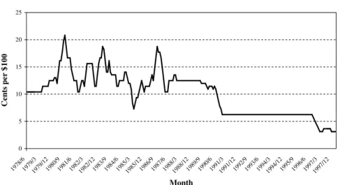
To provide evidence on the changes in liquidity and bid–ask spreads, we examine both the Treasury and corporate bond markets for the two sub-periods. For Trea- sury bonds, bid–ask spreads are available daily from the Wall Street Journal. We calculate the average bid–ask spread for the 10-year Treasury Note based on a sample of spreads from the last day of each month. The average spread is 13 cents per $100 over the 1978–1987 sub-period and 7 cents per $100 over the 1988–1998 sub-period.

Fig. 1 shows a 6-month moving average of the spreads using end-of-month data over the period January 1978 to March 1998. It is consistent with an increase in liquidity between the two sub-periods.

Unfortunately, data on bid–ask spreads in the corporate bond market were not available until recently, and then only for recent time periods. Hong and Warga (2000) and Schultz (2001) provide the first look at bid–ask spreads in the corporate bond market. Hong and Warga (2000) examine bid–ask data from the NYSEÕs ABS for October 1996 through February 1997 and from the National Association of Insurance Commissioners (NAIC) for the period from January 1995 through December 1997. The ABS provides data for an exchange market, while the NAIC provides data for the dealer market. They find the effective spreads on investment grade corporate bonds are similar across the two markets, with the spread on the exchange being 20.9 cents per $100 versus 13.28 cents per $100 in the dealer market. Schultz (2001) uses data from Capital Access International for the period from January 1995 through April 1997 and estimates a spread of 27 cents per $100 for investment grade corporate bonds. Interestingly, the lowest estimate is similar to the 13 cents per $100 in the Treasury market over the 1978–1988 sub- period.

(17)

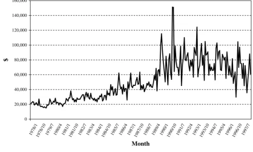
There is no data we are aware of that will allow us to estimate the bid–ask spread on corporate bonds during our earlier sub-period 1978–1987. Thus, to provide evidence on the possible increase in liquidity in the corporate bond market between the two sample periods, we obtained data from the Wall Street Journal on volume per issue traded, which is the total volume divided by the number of issues traded on the NYSEÕs ABS. Elton and Green (1998) use Treasury bonds to show that liquidity, bid–ask spreads, and trading volume are directly related. Thus, comparing volume in the corporate bond market in the two sub-periods may indicate changes in liquidity and in bid–ask spreads. Based on a sample from the last day of each month, the average volume per issue traded was $30,341 during the 1978–1987 sub-period versus $71,362 during 1988–1998 sub-period. Fig. 2 shows an upward trend in volume per issue traded over time, which is consistent with an increase in liquidity in the corporate bond market between the two sub-periods and implies that spreads likely declined as well.

Given the decline in liquidity, we divide the sample period into two sub-periods:

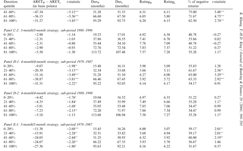
1978–1987 and 1988–1998.¹⁹ Table 2 reports the returns of the winner–loser portfolios for each sub-period. Consistent with the dealer inventory rebalancing explanation, the results for all strategies show significant reversals in the first sub-period and a substantial reduction in the second. For example, across all strategies, 25 of 30 generate reversals that are significant at the 5% level. The mean (median) loss is )30.05 ()26.62) basis points per month. In the second sub-period, only 4 of 30 strategies generate reversals that are significant at the 5% level. The mean (median)

0 5 10 15 20 25

1978/6 1979/3

1979/12 1980/9

1981/6 1982/3

1982/12 1983/9

1984/6 1985/3

1985/12 1986/9

1987/6 1988/3

1988/12 1989/9

1990/6 1991/3

1991/12 1992/9

1993/6 1994/3

1994/12 1995/9

1996/6 1997/3

1997/12

Month

Centsper$100

Fig. 1. Six-month moving average bid–ask spread on 10-year Treasury Note.

19The sub-period analysis for Treasury bond returns yields results similar to those found for the full sample period. The results suggest there are no reversals in any of the sub-periods across all six strategies for Treasury bond returns. It is clear that Treasury bond returns do not exhibit any cross-sectional serial covariance.

(18)

reversal for this sub-period is)3.31 ()4.39) basis points per month. These results are consistent with the existence of dealer inventory rebalancing, but not overreaction.²⁰ Perhaps this is not surprising given that corporate bond prices are derived from Treasury prices and bond characteristics, reducing the potential for overreaction to play a role in corporate bond pricing.

7.2. Gauging the relationship between bid–ask spreads and reversals

As a ﬁnal analysis, we use Eq. (1) and the bid–ask spreads for Treasury and Cor- porate bonds to determine the size of the reversals that may be induced by inventory cost considerations. In other words, we examine how bid–ask spreads translate into reversals, which are in the security-speciﬁc portion of bond returns. Table 3 shows the magnitude of the return reversals for various assumptions about the size of the bid–ask spread and the probability of a reversal, (p). The probability of reversal

0 20,000 40,000 60,000 80,000 100,000 120,000 140,000 160,000

1978/1 1978/10 1979/7 1980/4 1981/1 1981/10 1982/7 1983/4 1984/1 1984/10 1985/7 1986/4 1987/11987/10 1988/7 1989/4 1990/1 1990/10 1991/7 1992/4 1993/1 1993/10 1994/7 1995/4 1996/11996/10 1997/7

Month

$

Fig. 2. Volume per issue traded on NYSE ABS.

20In Section 5, we use liquidity as a screen for bonds that may suffer from data errors. The liquidity screen is cross-sectional and assumes that the data errors are somewhat constant across time. Thus, we eliminate those bonds that were the most illiquid in any given month to demonstrate that the reversals still exist when bonds that are most likely to suffer from data errors are eliminated. For example, eliminating the least liquid 25% of bonds might cause the average spread in the earlier sub-period to decline from 60 to 50 bps, while eliminating the least liquid 50% of bonds in the later sub-period might cause the average spread to decline from 25 to 20 bps. In the full sample period analysis, reversals with the liquidity screens are slightly smaller than those without the screens but remain significant. In Table 2, we examine reversals across two sub-periods and use lower bid–ask spreads (for example, 60 bps in the earlier period versus 25 bps in the later sub-period) over time as an explanation for the reduction in the reversals. Thus, the results in Section 5 and Table 2 are consistent.