Risk management strategies for banks

Risk management strategies for banks

Wolfgang Bauer

^a,b,*

, Marc Ryser

^c

aSwiss Banking Institute, University of Z€uurich, Plattenstr. 14, Z€uurich 8032, Switzerland

bRiskLab, ETH Z€uurich, Z€uurich, Switzerland

cECOFIN Research and Consulting, Z€uurich, Switzerland Accepted 18 November 2002

Abstract

We analyze optimal risk management strategies of a bank financed with deposits and equity in a one period model. The bank’s motivation for risk management comes from deposits which can lead to bank runs. In the event of such a run, liquidation costs arise. The hedging strategy that maximizes the value of equity is derived. We identify conditions under which well known results such as complete hedging, maximal speculation or irrelevance of the hedging decision are obtained. The initial debt ratio, the size of the liquidation costs, regulatory restrictions, the volatility of the risky asset and the spread between the riskless interest rate and the deposit rate are shown to be the important parameters that drive the bank’s hedging decision. We further extend this basic model to include counterparty risk constraints on the forward contract used for hedging.

2003 Elsevier B.V. All rights reserved.

JEL classification:G1; G21; G28

Keywords:Bank; Bank risk management; Corporate hedging

1. Introduction

The focus of this paper is to study the rationale for banks’ risk management strat- egies where risk management is defined as set of hedging strategies to alter the prob- ability distribution of the future value of the banks’ assets.

*Corresponding author. Tel.: +41-1-634-27-22; fax: +41-1-634-49-03.

E-mail addresses:wobauer@isb.unizh.ch(W. Bauer), marc.ryser@ecofin.ch (M. Ryser).

URL:http://www.math.ethz.ch/~bauer.

0378-4266/$ - see front matter 2003 Elsevier B.V. All rights reserved.

doi:10.1016/j.jbankfin.2002.11.001

www.elsevier.com/locate/econbase

There is a broad literature on these decisions for firms in general, beginning with Modigliani and Miller (1959): Their famous theorem states that in a world of perfect and complete markets, financial decisions are irrelevant as they do not alter the value of the shareholder’s stake in the firm. The only way to increase shareholder’s wealth is to increase value of the firm’s assets. Neither the capital structure nor the risk man- agement decisions have an impact on shareholder’s wealth.

Some important deviations from the perfect capital markets in the Modigliani–

Miller setting have been identified, giving motivations for firms to care about risk management, such as taxes, bankruptcy costs, agency costs and others (Froot et al., 1993; Froot and Stein, 1998; Smith and Stulz, 1985; DeMarzo and Duffie, 1995; Stulz, 1996; Shapiro and Titman, 1986). When these reasons for risk manage- ment are incorporated into the firm’s objective function, one finds the following basic result: When all risks are perfectly tradeable the firm maximizes shareholder value by hedging completely (Froot and Stein, 1998; Broll and Jaenicke, 2000; Moz- umdar, 2001).¹

However, the Modigliani–Miller-theorem as well as the aforementioned hedging motives are ex ante propositions: Once debt is in place, ex post financial decisions can alter the equity value by expropriating debt holders. This strategy is known as asset substitution (Jensen and Meckling, 1976). Because of limited liability, the posi- tion of equity holders can be considered as a call option on the firm value (Black and Scholes, 1973). This implies that taking on as much risk as possible is the optimal ex post risk management strategy. In summary, theory is inconclusive regarding the question of the optimal hedging strategy of firms.

Turning to the question of optimal hedging and capital structure decisions of banks, a first finding is that the analysis within the neoclassical context of the Modi- gliani–Miller-theorem would be logically inconsistent. Banks are redundant institu- tions in this case and would simply not exist (Freixas and Rochet, 1998, p. 8). The keys to the understanding of the role of banks and their financial decisions are trans- action costs and asymmetric information. These features have been dealt with exten- sively in the banking literature, departing from the neoclassical framework (Baltensperger and Milde, 1987; Freixas and Rochet, 1998; Merton, 1995; Schrand and Unal, 1998; Bhattacharya and Thakor, 1993; Diamond, 1984, 1996; Kashyap et al., 2002; Allen and Santomero, 1998, 2001):

• Banks have illiquid or even nontradeable long term assets because of the transfor- mation services they provide.

• Part of the illiquidity of banks’ assets can be explained by their information sen- sitivity; banks can have comparative informational advantages due to their role as delegated monitors. Examples include information about bankruptcy probabili- ties and recovery rates in their credit portfolio. This proprietary information

1This result is a consequence of the payoff-function’s concavity induced by the risk management motives and the application of Jensen’s inequality.

can be further improved through long term relationships with creditors (Boot, 2000; Diamond and Rajan, 2000).

• In contrast to other firms, banks’ liabilities are not only a source of financing but rather an essential part of their business: Depositors pay implicit or explicit fees for deposit-related services (i.e. liquidity insurance, payment services, storage).

The leverage in banks’ balance sheets is thus many times higher.

• Bank deposits can be withdrawn at any time. The sequential service constraint on these contracts and uncertainty about the bank’s ability to repay can lead to a

‘‘bank run’’ situation: All depositors rush to the bank at the same time to with- draw their money, trying to avoid being the last one in the waiting queue. This threat of bank runs creates an inherent instability for the bank’s business (Dia- mond and Dybvig, 1983; Jacklin and Bhattacharya, 1988).

These characteristics highlight the major differences between banks and other firms: Banks, in contrast to other corporations, are financed by deposits. Their ongo- ing operating value would be lost to a large extent in case of bankruptcy; depositors can immediately call their claims and run whereas illiquid and information sensitive assets have to be liquidated by fire sales at significant costs (Diamond and Rajan (2000, 2001); Shrieves and Dahl (1992); the size of bankruptcy costs of banks was estimated in James (1991)). However, these features of a bank are ignored by most of the literature on capital structure and hedging decisions, which usually deals with nonfinancial firms.

In a recent contribution, Froot and Stein (1998) developed a framework to ana- lyze a bank’s optimal capital allocation, capital budgeting and risk management decisions. Their motivation for the bank to care about risk management stems from convex costs of external financing for a follow-up investment opportunity. This in- duces the bank’s objective function to be concave (the authors call this internal risk aversion): The more difficult it is for the bank to raise external funds, the more risk averse it behaves. A publicly traded bank in an efficient and complete market does not reduce shareholder value by sacrificing return for a reduction in risk. Thus, risk reduction is always desirable for the risk-averse bank in the Froot and Stein (1998)- setting. Hence, the resulting optimal strategy is to hedge completely. However, the authors omit the equity’s feature of limited liability and the corresponding agency problems between shareholders and debtholders. Furthermore, since in their model, there is no depository debt and thus no bank run possibility, potential effects of de- faults on capital structure and risk management decisions are ignored.

In this paper, we model the hedging decision of a bank with the aforementioned characteristics. We assume the capital budgeting decision to be fixed. In a one-per- iod-two-states-model, the bank has a given amount of depository debt. The deposit rate contains a discount due to deposit-related services. The present value of this dis- count constitutes the bank’s franchise value. On the other hand, bank runs can force the bank to sell all of its assets at once, incurring significant liquidation costs. This creates an incentive for not having extraordinary high levels of depository debt. Fur- ther, we assume that the bank is restricted in its risk taking behavior by a regula- tor. We also incorporate limited liability for equity. We assume that the bank’s

management acts in the shareholder’s interest and maximizes the present value of the equity. It faces thus conflicting incentives for risk management: Regulatory restric- tions and liquidation costs in case of bank runs limit the risk taking on one hand.

On the other hand, limited liability creates incentives for risk taking. This setting al- lows us to identify situations in which well known results from the corporate finance literature are found: We show that for some banks, it is optimal to hedge completely as in Froot and Stein (1998). Other banks will take on as much risk as possible to aug- ment shareholder value by expropriating wealth from depositors, a strategy known as asset substitution (Jensen and Meckling, 1976). For still other banks, the risk manage- ment decision is shown to be irrelevant as in Modigliani and Miller (1959).

The remainder of this paper is organized as follows. In Section 2, we present the model, discuss the bank’s objective function and derive the optimal hedging strategy.

In Section 3, we discuss the impact of forward counterparty restrictions on the hedg- ing positions of the bank: Since depositors have absolute priority because of their possibility to withdraw at any time, the forward counterparty can face additional de- fault risk. It may therefore limit its contract size with the bank. Section 4 concludes the analysis and gives an outlook on further research possibilities.

2. The general model 2.1. The market

Let a probability space (X;F;P) be given, where we define X:¼ fU;Dg,

F:¼ f;;fUg;fDg;Xg and PðUÞ ¼p. The model has one period, between time

t¼1 andt¼2 andT f1;2gdenotes the set of time indices.

The market consists of two assets: A riskless asset has at timet¼1 a value nor- malized to 1,B₁¼1, andB₂¼B₁Rat timet¼2 whereR>1 is fixed and given; fur- ther, a risky asset with value P₁>0at time t¼1 and a valueP₂ðxÞ at timet¼2 where

P₂ðxÞ ¼ P_uP₁u; x¼U;

P_dP₁d; x¼D;

where we assume that

u>R>d: ð1Þ

For hedging purposes, we further introduce a redundant forward contract on the risky asset: It is entered at timet¼1 at no cost and the buyer of the contract has to buy one unit of the risky asset at time t¼2 at the forward price RP₁. Hence, the valuef_tof the forward contract is

f1¼0;

f₂ðxÞ ¼ fuPuRP1; x¼U;

f_d P_dRP₁; x¼D:

(

Since we have two assets with linearly independent payoffs and two states of the world, the market is complete. We define the unique risk neutral probabilityQby QðUÞ ¼:qsuch thatE^Q½^P_B²

2 ¼P₁, whereq¼^Rd_ud. 2.2. The bank

To derive the bank’s objective function, we make the following two assumptions that deal with agency problems: We explicitly exclude agency problems between shareholders and bank managers as their decision-taking agents. However, since banks empirically have very high debt levels, we take asset substitution as an agency problem between shareholders and depositors into account. Therefore, the problem of choosing risk after the choice of the initial capital structure is especially pro- nounced (Leland, 1998):

Assumption 1. Management’s compensation is structured to align the manager’s interests with those of the shareholders. Therefore the firm’s objective is to maximize the value of equity.

This objective is based on the completeness of the financial market. It is therefore possible to achieve any distribution of wealth across states. The Fisher separation theorem then states the following: All utility maximizing shareholders agree on the maximization of firm value as the appropriate objective function for the firm, not- withstanding the differing preferences and endowments (Eichberger and Harper, 1997, p. 150). However, as Jensen and Meckling (1976) pointed out, shareholders in levered firms can do better behaving strategically. They will prefer investment or hedging policies that maximize the value of only their claim, if they are not forced to a precommitment on the investment and hedging strategy.

Assumption 2. When setting its capital structure, the bank cannot precontract or precommit its hedging strategy. It will choose the hedging strategy ex post, after deposits have been raised.

At timet¼1, the bank has a loan portfolio, which has the same dynamics as the risky asset. Its value att¼1 equals aP1, we will thus say it has a prior position of a>0units of the risky asset.²The bank has two sources of capital: Depository debt and equity where the latter has limited liability. The initial amount of depository debt D₁ is given. While it would also be interesting to analyze the bank’s capital structure decision, we limit our analysis to the hedging policy, assuming that the bank has already set its target capital structure.

2Through their monitoring activity, banks may be able to generate additional rents on the asset side as well. These proprietary assets are however often not tradeable. In this situation, the market is incomplete.

This incompleteness creates problems for the determination of a unique objective function for the bank and we leave the analysis of the case with nontradeable proprietary assets for further research.

2.3. The deposits and the run-threat to equity

In most papers dealing with the capital structure of firms in general, the tax- advantage of debt is a main incentive for firms to carry debt. For banks, however, there is a more important motivation for carrying depository debt. Depository debt in banks can be regarded as a real production element (Bhattacharya and Thakor, 1993). Due to deposit-related services (liquidity provision, payment services), the de- posit rate will be lower than the rate that fully reflects the risk. We assume that the bank gets a discount of s>0on the deposit rate, resulting in

D₂¼D₁R_D;

whereR_D>1 is the deposit rate net of the discount that the bank receives. We call the net present value of these discounts from future periods the franchise value of the deposits, denoted byFV_t,t2T:

FV₁¼sD1

B₂ ; FV₂¼0;

where^sD_B¹

2 ¼E^Q½_B^s1₂.

Because of its significant influence on the bank’s equity payoff, we should high- light another important difference between bank deposits and traded debt: Asset-re- turn shocks affect market prices of traded debt equally over all debt holders, whereas the nominal amount of deposits can be withdrawn at any time. However, as Diamond and Dybvig (1983) pointed out, the sequential service constraint on these fixed-commitment contracts along with sudden shocks in the liquidity needs of depositors can lead to a situation in which all depositors withdraw their money at the same time. This is because the amount received by a individual depositor solely depends on his relative position in the waiting queue. Such a bank run can happen as a ‘‘sunspot phenomenon’’, whenever there is a liquidity shock and even in the ab- sence of risky bank assets.³When uncertain asset returns are introduced into the analysis, there is another reason why bank runs can occur: Whenever the value of the bank’s assets is not sufficient to repay every depositor’s full claim, all fully in- formed rational depositors would run to the bank at the same time and cause a so-called information based bank run (Jacklin and Bhattacharya, 1988).

Let us assume that there arendepositors with equal amounts ofD₂=nof deposits.

We denote byV_Lthe critical asset value below which there will be a bank run. With- out liquidation costs, we find that V_L ¼D₂. Indeed, whenever the value V₂ of the bank’s assets at timet¼2 exceeds the nominal depositsD₂, all depositors will receive their nominal claim. But as soon as the valueV₂of the bank’s assets falls below the

3The right to withdraw at any time is an essential prerequisite for the efficiency of the deposit contract.

In accordance with Diamond and Rajan (2000), we therefore exclude the possibility of suspension of convertibility for the bank in our model; the bank cannot deny redemption of deposits as long as there are any assets left.

nominal valueD₂of the deposits, not all depositors can withdraw their full nominal amount anymore. In the latter case, each depositor faces the problem of choosing between two compound lotteries: By running, he chooses the lotteryL^Rwith payoffs depicted in Fig. 1. By not running, he chooses the lotteryL^NR with payoffs also de- picted in Fig. 1:

• When there is a bank run, the firstV₂=D₂percent of the depositors in the waiting queue receive their full nominal deposit D₂=n. Thus, if the individual depositor runs, the likelihood of arriving early at the queue (denoted Ôearly’) is V₂=D₂. The payoff in this case is ^D_n². If he joins the queue in a later position (denoted

’late’), his payoff is 0. When there is no bank run, the individual depositor is the only to run and he receives his nominal deposit D2=n or all of the assets remaining.

• When the individual does not run he either receives 0if there is a bank run or^V_n²if there is no bank run because in this case the value of the remaining assets is dis- tributed equally among the depositors.

ForV₂<D₂, the payoffs of the run-strategyL^Rare higher or equal to those of the no-run-strategy in all states of the world. Equivalently, the distribution of the run- strategyL^R first-order stochastically dominates the distribution of the no-run-strat- egyL^NR. Hence, every expected utility maximizing depositor with positive marginal utility will prefer the run-strategyL^R (see e.g. Mas-Colell et al., 1995). This leads to an equilibrium situation which is called information-based bank run.

In run situations, fire sales of assets necessary to pay out the depositors may create significant liquidation costs (indirect bankruptcy costs) on the other hand (Diamond and Rajan, 2001): Asset market prices can drastically decline if big blocks of assets have to be sold immediately. If the bank has to sell all of its assets at once during a run, we assume that there are liquidation costs ofcV2, 0<c<1. The fractioncof firm value lost in case of bank runs creates a major incentive for the bank to hedge its risk: Averaging 30% of the bank’s assets, these losses are substantial in bank fail- ures as James (1991) found in his empirical work.

Since there is always a possibility of ‘‘sunspot’’-bank runs due to unexpected liquidity shocks, the individual depositor is uncertain whether there will be a bank

Fig. 1. Payoffs to a depositor in absence of liquidation costs.

run at timet¼2 (Diamond and Dybvig, 1983).⁴Because of this uncertainty and the liquidation costscV2,V_L, the value of the assets below which an information based bank run will be triggered, shifts to

V_L¼ D2

1c; ð2Þ

forD₂<V₂< ^D2

1cwe now have the payoffs given in Fig. 2. They resemble the payoffs shown in Fig. 1 without liquidation costs, but now total value of the assets is reduced to ð1cÞV2 instead ofV₂in situations of bank runs:

• When there is a bank run, the firstV₂ð1cÞ=D2 percent of the depositors in the waiting queue receive their full nominal depositD₂=n. If the individual depositor runs, the likelihood of arrivingÔearly’ isV₂ð1cÞ=D2and the payoff in that case is

D2

n. If he joins the queue in a later position (denotedÔlate’), his payoff is 0. When there is no bank run, the individual depositor is the only one to run and he re- ceives his nominal depositD2=n or all of the assets remaining.

• When the individual does not run, he receives 0if there is a bank run. Otherwise he either receives his full nominal amount^D_n²(ifD26V26VL), or a fraction^V_n²of the remaining assets, which are distributed equally among the depositors.

Again, forV₂< ^D2

1c, the distribution of the run-strategy L^R first-order stochasti- cally dominates the distribution of the no-run-strategy L^NR, causing an informa- tion-based bank run equilibrium.

Without this bank run-threat, the payoff function for the bank’s equity at time t¼2 would be

SðV2;D2Þ V2D2; V2PD2; 0; 06V2<D2: (

Fig. 2. Payoffs to a depositor in the presence of liquidation costs.

4We assume that the bank can only raise deposits of the sizeD16ð1cÞaP1such that bank runs at timet¼1 are excluded. This condition can equivalently be written as_aP^D1

1

6ð1cÞand interpreted in the following way: Banks can only raise deposits up to the point where the debt ratio equals the recovery rate in case of a run.

This is the payoff of an ordinary call option on the firm value with strikeD2. How- ever, in the presence of liquidation costs, a bank run will always take place ifV2<VL. Thus the residual payoff to shareholders drops to zero belowV_L. SinceV_L>D₂, the equity payoff changes to

SðV2;D₂Þ V₂D₂; V₂PV_L; 0; 06V₂<V_L;

ð3Þ as shown in Fig. 3.

2.4. The optimization problem

At timet¼1, the bank chooses a hedging position consisting ofhunits of the for- ward contract on the risky asset. As a function of the chosen hedging positionh, the value of the bank’s assets at timet¼1 hence is

V₁ðhÞ ¼aP1þhf₁þFV₁; h2R; ð4Þ and the value of the bank’s assets in stateU andDrespectively at time t¼2 for a given hedging positionh is denoted by

V_uðhÞ aPuþhf_u; h2R; ð5Þ

V_dðhÞ aPdþhf_d; h2R: ð6Þ

To study the impact of regulatory or other restrictions on the risk management, we introduce lower and upper bounds⁵on the hedging positionh,

Fig. 3. Payoff function of equity.

5Liquidation costscV2are expressed as a fraction of the final firm valueV2. Thus, by introducing the following (merely technical) restriction on the bank’s hedging decision, admitting only hedging strategies for which the firm value is always positive, we guarantee nonnegative liquidation costs. This amounts to the restriction h2 ½Z^u;Z^d where Z^u a_uR^u and Z^d a_dR^d . Indeed, these constants follow from solving the inequalitiesVuðhÞP0andVdðhÞP0using the definitions (5) and (6) of VuðhÞand VdðhÞ.

V^uðhÞP0holds forh2 ½Z^u;1ÞandV^dðhÞP0holds forh2 ð1;Z^d, thus nonnegative firm value is the outcome for hedging strategies inð1;Z^d \ ½Z^u;1ÞÞ. It follows from the definition ofZ^uthatZ^u<a thusaas the lower bound of the set of feasible hedging positions guarantees nonnegative firm value in stateU. Throughout the following we assume that the upper bound is more restrictive thanZ^d,a1<Z^d.

a6h6a₁: ð7Þ The lower bound a is equivalent to a no net-shortsales-constraint.⁶

The payoffSto shareholders at liquidation at timet¼2 is a function of firm value and deposits,SðV2;D₂Þ. Since the financial market is arbitrage-free and complete, the present value of equity at timet¼1 for a given future valueV₂of the assets equals

E^Q SðV2;D₂Þ B₂

:

The bank’s management’s goal is to maximize the present value of equity at time t¼1, by choosing a hedging positionh. Let

IðhÞ E^Q SðV2ðhÞ;D₂Þ B2

ð8Þ denote the objective function.IðhÞis the value of equity at timet¼1 as a function of the hedging portfolioh. Then, the bank’s optimization problem at timet¼1 is

amax6h6a1

IðhÞ ¼ max

a6h6a1

E^Q SðV2ðhÞ;D2Þ B₂

¼ max

a6h6a1

E^Q SðaP2þhf2;D2Þ B₂

: ð9Þ

2.5. Optimal hedging strategy

The present value of equity as a function of the hedging positionh,IðhÞ, has the following form, depending on whether for a given hedging positionhthere will be a positive payoff to shareholders in both statesUandD or only in stateU:

1. For hedging positionshsuch that the assets’ total value exceeds the bank run trig- gerV_L in both statesUandD,V_uðhÞ>V_L andV_dðhÞ>V_L, amounting to a positive payoff to shareholders in both states (we call these hedging portfolios portfolios of type 1), the objective function is

IðhÞ ¼ q

B₂½aPuþhðPuRP1Þ D2 þ1q

B₂ ½aPdþhðPdRP1Þ D2:

2. For hedging positionsh such that the assets’ total value exceeds only in stateU the bank run trigger V_L,V_uðhÞ>V_L, but is smaller than V_L in state D,V_dðhÞ<V_L (that is, there is a bank run in state D and shareholders receive only in stateU a positive payoff; we call these hedging positions portfolios of type 2), the objec- tive function is

IðhÞ ¼ q

B₂½aPuþhðPuRP1Þ D2:

6The net position in the risky asset is restricted to be nonnegative and thus, the cases where V_uðhÞ<V_dðhÞcan be omitted.

Thus, in order to solve the optimization problem, we need to find conditions which guarantee the existence of hedging positions h of either type 1 or type 2 for a given market and bank structure.

Lemma 1.The payoff to shareholders is positive in stateU for hedging positionsh hPV_LaPu

P_uRP₁¼:K^u: ð10Þ

The payoff to shareholders is positive in stateDfor hedging positionsh h6VLaPd

P_dRP₁¼:K^d: ð11Þ

K^uis the minimal hedging position for which shareholders receive a positive pay- off in stateU.K^d is the maximal hedging position for which shareholders receive a positive payoff in state D. Hence, the portfolios of type 1 are in the set ½K^u;K^d. Therefore, the relationship among the termsK^uandK^d will determine whether this set is empty and whether there are hedging positions of type 1 or only of type 2.

Corollary 1.Hedging positions hof type 1 exist if

V_L6aP1R¼:V: ð12Þ

V is the value of the assets of theÔfully hedged bank’ at timet¼2, i.e. the value attained if the bank sells forward its whole positionain the risky asset and the future value becomes certain, VuðaÞ ¼VdðaÞ ¼aP1R¼V. Thus, if the bank run trigger V_Lis smaller or equal to the forward priceV of the bank’s prior position, there exist hedging positions for which shareholders receive a positive payoff in both states U and D. It is obvious that the fully hedged position a would be such a position.

And if the payoff to shareholders with this forward position is strictly positive, there will be other forward positions close to a which also yield a positive payoff to shareholders. Otherwise, if the forward priceV of the bank’s prior position is smaller than the bank run triggerV_L then there are only hedging positions of type 2. Share- holders then receive a positive payoff only in stateU and a zero payoff in state D, V_uðhÞPV_L andV_dðhÞ<V_L.

The shape of the objective function is further clarified by the following Lemma 2.IfV_LPV, then the inequality

K^d6a6K^u ð13Þ

holds. Otherwise, ifVL6V, then the inequality

K^u6a6K^d ð14Þ

holds.

The intuition for (13) and (14) is as follows:

• IfV_L>V, then the fully hedged positiona, leading to a value ofV in both states of the world, results in a payoff of zero to shareholders, since the firm value is in this case below the bank run triggerV_L. Thus, the minimal (maximal) hedging po- sition at which shareholders receive a positive payoff in stateU(D), i.e.K^u ðK^dÞ, would be higher (smaller) thana. This corresponds to (13).

• The converse holds ifVPV_L. Then the fully hedged positionayields a positive payoff to shareholders. Then the minimal (maximal) hedging position at which shareholders receive a positive payoff in stateU(D), i.e.K^u(K^d), would be smaller (higher) thana. This corresponds to (14).

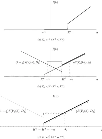
Fig. 4 displays the objective functionIðhÞwith the no net short sales restriction in the three cases where V_L>V (Fig. 4(a)), V_L<V (Fig. 4(b)) and V_L ¼V (Fig. 4(c)).

The bold line is the feasible part of the objective function.

Fig. 4. Three types of objective functions with no net short sales restrictions.

Proposition 1

1. If the forward price of the bank’s prior position is less than the bank run trigger, aP1R<V_L, and if there is a positive payoff to shareholders in stateUat the maximal admissible hedging position,a₁PK^u, then the optimal hedging position is

h¼a1:

2. Otherwise, ifaP1R>V_L, we find the following optimal hedging strategies:

(a) Ifa₁PK^d anda₁>J_u, then h¼a₁, whereJ_u is defined by (15) below.

(b) IfJ_u>a₁>K^d, thena6h6K^d. (c) Ifa₁<K^d, thena6h6a₁.

3. IfaP1R¼V_L, we find the following optimal hedging strategies:

(a) Ifa₁<J_u, thenh¼ a.

(b) Ifa₁>J_u, thenh¼a₁.

J_u can be characterized as follows (see Fig. 4(b)): The positionh¼J_ubelongs to the set of hedging positions for which the objective function is increasing; further,J_u is the position for which the value function equals the value that is attained on the set where the objective function is constant,

J_u

aP1D2

R qðaPuD2Þ R qP1ðuRÞ

R

: ð15Þ

The three optimal hedging decisions in Proposition 1 have the following economic interpretation:

• h¼a1 is the strategy of maximal speculation.

• h¼ ais the case of complete hedging where the bank sells forward its whole ini- tial position.

• In the case whereK^u<K^d, the bank is indifferent between the hedging strategies in the rangeK^u6h6K^d.

Part 1 of Proposition 1 covers the case in which the payoff to shareholders would be zero if the bank hedged completely. It is the case in which the forward price of the prior position is less than the bank run trigger,V <V_L. If a positive payoff to share- holders in stateUis attainable by taking on more risk,a₁PK^u, we have a ‘‘gamble for resurrection’’-situation: It is always optimal to take as much risk as possible, h¼a₁. The conditionV_L >V can equivalently be written as

D₁=aP1>ðR=RDÞð1cÞ; ð16Þ

which says that the initial debt ratio is higher than the recovery rate (in case of a run) multiplied by the spread between the deposit rate and the riskless interest rate.

Hence, for banks with high initial debt ratio and/or high liquidation costs, it is al- ways optimal to gamble for resurrection.

Parts 2a to 2c of Proposition 1 cover the cases in which shareholders would still receive a positive payoff if the bank hedged completely, V_L <V, resp. D₁=aP1<

ðR=RDÞð1cÞ.

• In 2a, the maximal admissible hedging positiona₁yields a higher expected payoff than theÔfully hedged’ positiona. Since shareholders could lock in a sure posi- tive payoff by hedging completely, this is not a ‘‘gamble for resurrection’’, although the optimal hedging strategy is the same. Due to equity’s nonlinear pay- off, they can expropriate wealth from depositors by taking on more risk: The in- crease of the payoff in stateUovercompensates the liquidation costs in state D.

This strategy is known as asset substitution (Jensen and Meckling, 1976). Hence, in the current model, banks in this situation have loose regulatory or other restric- tions (a largea₁). They can take that much risk that the bank run threat does not have a disciplinary effect anymore.

• In 2b, the risk management restriction is so constraining, that at the maximal admissible positiona₁, the gain in expected return does not outweigh the expected liquidation costs of this portfolio. The expected payoff to shareholders for this hedging position is smaller than for theÔfully hedged’ positiona. However, there is no unique optimal hedging strategy: Shareholders are indifferent with respect to the hedging strategies in the whole range betweenaand K^d. If the initial debt ratio_aP^D1

1 is higher than _R^d

Dð1cÞ, then K^d<0and the optimal hedging strategy is risk reducing,h<0. Risk reducing banks in this case are those with a high ini- tial debt ratio, high asset volatility and/or high liquidation costs.

• In 2c, the maximal admissible hedging position a1 belongs to the portfolios for which shareholders receive a positive payment in both states U andD. The ex- pected payoff is the same as the one of theÔfully hedged’ positiona. In this case, the Modigliani–Miller-result of hedging-irrelevance also holds ex post, after the determination of the capital structure: Shareholders are indifferent with respect to all admissible hedging strategies. Banks in this case are, however, forced to- wards a safe behavior: The risk management restrictions prevent asset substitu- tion since they guarantee that the value of banks’ assets can never fall below the bank run trigger.

In part 3a, theÔfully hedged’ positionh¼ a is optimal. Any risk taken by the bank induces liquidation costs. But the expected return cannot be increased suffi- ciently such that the shareholders would receive a higher expected payment at least in one state since J_u>a1>K^d. Banks in this situation do not have any risk toler- ance. They cannot improve the shareholders’ position by asset substitution. In our model, only for this special situation, the Froot and Stein (1998)-result of complete hedging is derived as the unique optimal hedging strategy.

In part 3b, the regulatory constrainta1is loose enough to allow the bank to take on enough risk such that the expected return again outweighs the expected liquida- tion costs.

Overall, for a regulatory restricted bank financed with deposits that is subject to liquidation costs in the event of bank runs, the common interpretation of equity as a

call option does not necessarily apply: Equity value is not always increased by an in- crease in asset-risk. Further, higher liquidation costs lead to an increase of the bank run trigger. This creates larger downside risk for shareholders that cannot always be outweighed by a higher expected return, because regulatory restrictions place an upper limit on risk taking.

On the other hand, depending on how much risk taking regulatory or other restrictions allow, hedging completely as in Froot and Stein (1998) is almost never the unique optimal hedging strategy: Over a wide range, all hedging positions can be equally optimal. Risk shifting to depositors is optimal as long as the higher ex- pected return outweighs the possible downside loss. If risk management restrictions are set to prevent asset substitution, the value of the bank’s assets cannot fall below the bankrun trigger. The result then coincides with the Modigliani–Miller-result of hedging irrelevance.

3. Impact of counter party risk constraints

We extend the analysis of the previous section by introducing counter party restrictions on the attainable forward contract size used for hedging. The forward price RP₁ is set such that expected profit from the forward contract is zero under the risk neutral probability measureQ. Yet, if the bank can default on the forward contract, the counter party will demand a higher forward price to get compensated for the additional risk. If we leave the forward price fixed, the bank will not be able to enter every desired forward position any more. The counter party restricts the hedging decision by offering only forward contracts for which the probability of de- fault does not exceed some threshold. In the current binomial setting, statements on probabilities correspond to conditions on statesUandD:

• Zero probability of default is equivalent to no default in both states UandD.

• If the probability of default can be positive, then the bank is not allowed to default either in stateU or in stateD.

Proposition 2.The bank will not default on the forward contract in state U for con- tracts of sizehPK^u. Further, the bank will not default on the forward contract in state Dfor contracts of sizeh6K^d. Under the requirement that the bank should not default in any state of the world on its obligations from the forward contract, it will not be able to enter a forward contract unlessK^u6K^d. It will only be offered contractshsuch that K^u6h6K^d.

The question when the bank is offered both long and short or only long or only short positions is answered by the following

Lemma 3.If the bank is not allowed to default in stateU(stateD), it will be offered short (long) positions if and only if V_L<aP1uðVL<aP1dÞ.

Hence, the restriction not to default in stateDmay prevent the bank to enter long positions, namely if D₁=aP1>ð1cÞðd=RDÞ. These banks either have a high debt ratio, high liquidation costs and/or a high asset-volatility. They would face a bank run in stateDwithout hedging and the costs would be borne by the counter party.

On the other hand, the restriction not to default in stateUmay prevent the bank to enter short positions ðif D₁=aP1>ð1cÞðu=RDÞÞ. The debt ratio, the liquidation costs and/or the asset-volatility of these banks is that high that they would face a bank run already in theÔgood’ state of the worldU and the counter party enforces the asset substitution in this case. The most important type of restriction⁷is the one which does not allow default in any state. In the case whereVL>V,⁸the bank can- not enter a forward contract. With its combination of deposits, initial position and liquidation costs, it will not be offered forward contracts due to default risk. Thus, the gamble for resurrection is not possible any more. WhenV_L6V, the bank is pre- vented from taking on any risk which would trigger a bank-run. It can only enter posi- tions in the forward in the rangea6h6K^d. Thus, the bank will always have the possibility to reduce risk by entering short positions. In the subcase where V_L>aP1d, it will not be able to obtain long positions (Lemma 3). That is, when the bank’s prior position is sufficient to prevent a bank run only in state U, but not in stateD, the bank will only be offered contracts that reduce the risk sufficiently to en- sure that there will be no bank run in stateD. Without hedging, the bank would face a bank run in stateD. But with the positive cash flowðPdRP₁Þfrom the short posi- tion in the forward contract in stateD, the bank’s assets are sufficient to prevent a run in stateD. The following Lemma tells when the bank will choose to hedge.

Lemma 4. In the case where VL6V andaP1d <VL, the bank will choose to hedge if D26aP1d <VL; ifaP1d<D2, then it is optimal for the bank not to hedge.

The reason for this hedging-strategy is the following: By hedging when D₂6 aP1d<V_L, the bank can preserve asset value in the down state D, that otherwise would be completely lost for the shareholders as liquidation costs. On the other hand, ifaP1d<D₂, all the remaining asset value up toD₂goes to the depositors anyway. If the bank hedges, it thus sacrifices some payoff to shareholders in stateUin exchange

7The constraint that the bank should not default in stateUbut is allowed to default in stateDis only meaningful if the risk neutral probability of stateD is very low. The forward contract price is then approximately not affected by the additional default risk. The following results then apply: IfVL>V, the bank can obtain only positionshPK^u, since it would default in stateUon all other positions. Therefore, the bank can still follow a strategy of asset substitution by holding long positions in the forward contract.

If evenVLPaP1u, that is, if the bank faced a bank run without hedging in stateU, it would only be offered long positions to hedge and thus be forced toÔgamble for resurrection’: For sufficiently large hedging positions, the value of the bank’s asset is above the bank run trigger in stateU(whereas in stateD, the bank will default on its obligation from the forward contract). In the case whereVL6V, the constraint that the bank is not allowed to default in stateUis not binding: It will be offered any contracts of sizehPK^u but the lower bound on its hedging positionhalready isawherea6K^u((14) in Lemma 2).

8V_L>V impliesK^d<K^u, and if follows from Proposition 2 that the bank will not be offered forward contracts.

for securing payoffs for depositors in stateD. The bank can do better for the share- holders by not hedging at all, that is, by keeping the higher expected return of the un- hedged position while letting the depositors bear the downside loss in stateD.

Overall, the introduction of counterparty-restrictions mitigates risk taking incen- tives for a bank, since it is not possible to gamble for resurrection anymore.

4. Conclusion

We have presented a one-period model in which we analyze the bank’s risk man- agement decision. The bank is regulatory restricted, financed by deposits and is sub- ject to liquidation costs in the event of a bank run.

We find that the common interpretation of equity as an ordinary call option does not apply: Equity value is not always increased by increasing the asset’s volatility, since this also raises the likelihood of a bank run. Whenever the expected costs of such a run for shareholders cannot be outweighed by an increase of the expected re- turn (because regulatory restrictions limit the maximum achievable risk), it is not optimal to take as much risk as possible. In these cases, safe banks with low debt ratios and asset volatility can still augment their risk exposure to the point where downside loss comes into play. However, for banks with a high debt ratio and a high asset volatility, risk reduction is the optimal strategy.

This deterrence of asset substitution however vanishes in the absence of regulatory constraints or with a complete deposit insurance (Calomiris and Kahn, 1991): With- out the possible downside loss, the equity payoff would be that of an ordinary call option and it would always be optimal for the bank to take as much risk as possible.

Also, without regulatory restrictions, the possible downside loss could always be out- weighed by higher expected return through higher risk-exposures.

On the other hand, depending on how much risk taking regulatory or other restrictions allow, it may not be optimal for the bank to hedge completely as in Froot and Stein (1998): Because equity features limited liability, risk shifting to depositors is still preferred as long as the higher expected return outweighs the possible down- side loss. The less restrictive regulatory restrictions are, the more relevant becomes this strategy of asset substitution. Without any restrictions of regulators or counter parties, asset substitution would always be the optimal strategy.

Further, there is one constellation for which the hedging decision is shown to be irrelevant, which coincides with the result of the Modigliani–Miller-theorem. This, however, is only a special situation, where the risk management restrictions, the size of the liquidation costs in case of a bank run and the initial debt ratio are all set such that risk shifting to depositors is impossible and no bank run takes place.

Among the open questions remains the analysis of the hedging decision in a mul- tiperiod setting. Bauer and Ryser (2002) have looked at the effect that the bank’s franchise value of deposits then has. It gives an incentive to reduce risk taking since the whole stream of future income from deposit services would be lost in a run sit- uation. Furthermore, it would be interesting to analyze the hedging decision in the presence of a nontradeable proprietary bank asset that generates an extra rent as

in Diamond and Rajan (2000). The market completeness breaks down in this case and the determination of a unique objective function for the bank is not trivial any- more.

5. Proofs

Proof of Lemma 1. Using the definition (5) ofV_uðhÞwe find that for a givenh V_uðhÞ>V_L()h>V_LaPu

P_uRP₁¼K^u; similarly for a given h

VdðhÞ>VL()h<V_LaPd

P_dRP₁¼K^d:

Proof of Corollary 1.From Lemma 1 we know thatV_uðhÞ>V_L forh2 ½K^u;1Þand V_dðhÞ>V_L for h2 ð1;K^d. Hence, hedging positions h of type 1 (that is, h for which bothV_uðhÞ>V_L andV_dðhÞ>V_L) areh2 ½K^u;K^d; this interval is not empty if

K^u6K^d: ð17Þ

Using the definitions (10) and (11) ofK^uandK^d this can be written equivalently as

VLaPu PuRP1

6^VLaPd

PdRP1. Solving forV_L yieldsV_L6aP1R¼V.

Proof of Lemma 2.Consider first the caseV_L>V. From the definition (12) follows V_LPV ¼aP1R. Subtracting aPu yields V_LaPuP aðPuP₁RÞ, dividing by ðPuP₁RÞ yields K^uPa. The inequalities forK^d and for the case where V_L6V follow in the same way. h

The following lemma will be useful to prove Proposition 1.

Lemma 5. The sets of candidates for the optimal hedging strategyharefa1g,fag and ð1;K^d \ ½K^u;1Þ. The values of the objective function evaluated at these can- didate points are

Iða1Þ ¼

q

B2½aPuþa₁ðPuRP₁Þ D₂; K^d6K^u6a₁ or K^u6K^d<a₁; aP1^D_B2²; K^u6a₁6K^d;

0; K^d <a₁<K^u;

8<

:

ð18Þ IðaÞ ¼ aP1^D_B²

2; K^u<K^d; 0; K^d<K^u;

ð19Þ

IðhÞ ¼ aP1^D_B²

2; K^u6h6K^d; 0; K^d <h<K^u:

ð20Þ

Proof of Lemma 5.For convenient notation, we write the constraints (7)a6h6a₁ in the form

Ah6a; ð21Þ

whereA ðA₁ A₂Þ⁰¼ ð1 1Þ⁰anda ða₁ aÞ⁰.

We consider first the caseV_L6V ¼aP1R. FromV_L<V ¼aP1Rand (17) follows thatK^u6K^d. Hence, for anyh2 ½K^u;K^dholds thatV_uðhÞPV_L andV_dðhÞPV_L. On this interval, the Lagrangian is as follows:

Lðh;l₁;l₂Þ ¼ q

B₂½aPuþhðPuRP1Þ D2 þ1q

B₂ ½aPdþhðPdRP1Þ D2 þX²

k¼1

l_kðAkha_kÞ

¼ ðaþhÞP1hP₁ B₁ D₂

B₂þX²

k¼1

l_kðAkha_kÞ;

yielding the first-order conditions oL

oh ¼P1P₁ B1

þX²

k¼1

l_kAk¼0; ð22Þ

oL

ol_k ¼A_kha_k ¼0; k¼1;2:

We have the following candidate points for an optimum:

1. l₁¼l₂¼0: (22) reduces to the condition P1_B^P1

1¼0where the last equality is due toB1¼1. Thus, in this case anyhsuch thatV_uðhÞPV_LandV_dðhÞPV_Lis opti- mal, that is, the set of candidates is½K^u;K^d. FromB1¼1 followsIðhÞ ¼aP1^D_B²

2, K^u6h6K^d.

2. If l₁6¼0, l₂¼0then h¼a1. Then, if K^u<K^d<a1 Iða1Þ ¼_B^q

2½aPuþ a₁ðP_uRP₁Þ D₂since the payoff to shareholders is zero in state D for h¼a₁ due to the fact thatK^d<a₁. IfK^u6a₁6K^d

Iða₁Þ ¼ q B2

½aPuþa₁ðP_uRP₁Þ D₂ þ1q B2

½aPdþa₁ðP_dRP₁Þ D₂

¼aP1D₂ B2

:

3. Ifl₁¼0,l₂6¼0thenh¼ a. Then, sinceK^u6a6K^d, IðaÞ ¼ q

B₂½aPuaðPuRP₁Þ D₂ þ1q

B₂ ½aPdaðPdRP₁Þ D₂

¼aP1D2

B₂:

Consider now the caseV_L>aP1Rwhen there are onlyhsuch thatV_uðhÞ>V_Land V_dðhÞ<V_L holds for fixedh. The Lagrangian is then

Lðh;l₁;l₂Þ ¼ q

B₂½aPuþhðPuRP₁Þ D₂ þX²

k¼1

l_kðAkha_kÞ;

yielding the first-order conditions

oL oh ¼ q

B2

½P_uRP₁ þX²

k¼1

l_kA_k ¼0: ð23Þ

We have the following candidate points for an optimum:

1. l₁¼l₂¼0could hold only if^P_P^u

1¼Rwhich was excluded in (1).

2. l₁6¼0,l₂¼0andh¼a1. Then, ifK^d<K^u6a1,Iða1Þ ¼_B^q₂½aPuþa1ðPuRP1Þ D₂since the payoff to shareholders is zero in stateDdue to the fact thatK^d<a₁. IfK^d<a₁<K^u we haveIða₁Þ ¼0since the payoff to equity holders is both zero in stateD (fromK^d<a₁) and in stateU(from a₁<K^u).

3. l₁¼0,l₂6¼0andh¼ a. Then, it follows thatIðaÞ ¼0since it follows from (13) thatK^d<aand hence at the positionashareholders receive a zero payoff in stateD.

As for the last equality, it is obvious that forh>K^d, the payoff to shareholders is zero in stateDand forh<K^u, the payoff to shareholders is zero in stateU, hence for K^d <h<K^ufollowsIðhÞ ¼0. h

Proof of Proposition 1.We consider first part 1 of the proposition, that is, the case whereVL>aP1Randa1PK^u. As this is the case whenK^d<K^u, it follows from (20) that the objective function equals zero for allh2 ðK^d;K^uÞincludinga(since, from Lemma 2, K^d<a<K^u). Definition (10) of K^u yields for a₁PK^u a₁P^V_P^LaPu

uRP1 or aPuþa₁ðP_uRP₁ÞPV_L. From (18), Iða₁Þ ¼_B^q₂½aPuþa₁ðP_uRP₁Þ D₂>0since V_L>D₂, hence, a₁ is the optimum.

We now turn to parts 2 and 3 of the proposition; both cases are covered by the inequality V_L6aP1R or equivalently K^u6K^d, 2 being the case of strict inequality and 3 the case of equality. Consider first 2a and 3b respectively. From (20) follows that forh2 ½K^u;K^d(and hence also forh¼ a)IðhÞ ¼aP1^D_B²

2. From J_u<a₁ fol- lowsaP1^D_B²

2<_B^q

2½aPuþa₁ðPuRP₁Þ D₂ ¼Iða1Þ, henceh¼a₁. Similarly follows for 2b and 3a whenJu>a1>K^dthataP1^D_B²

2 >_B^q

2½aPuþa1ðPu RP₁Þ D₂ ¼Iða₁Þ, henceh2 ½a;K^d.

In part 2c, feasible portfoliosh areh2 ½a;a₁ ðK^u;K^dÞ. Hence, from (20), all feasible portfolios have the same value of the objective function, IðhÞ ¼aP1^D_B2², K^u<h<K^d,h2 ðK^u;K^dÞ. h