Many fond memories belong to past and present members of the Morari research group: H. The conditions under which some of the new criteria reduce to the previously published measurement criteria are derived.
List of Figures
List of Tables
Chapter 1 Introduction
- Motivation
When one or more of the above factors make the design of an effective feedback control system based on the primary measurements alone infeasible, "secondary measurements" (that is, measurements of other process variables) should be used. Successful feedback control using secondary measurements depends on two major tasks: the selection of secondary measurements and the design of the inferential control system.
Sampling
Industrial Applications
- Distillation Columns
- Packed-Bed Reactors and Other Chemical Processes
- Pulp Digesters
For reliable, efficient control of the Kappa number, secondary process variables such as PH number, conductivity and digester liquid temperature can be used for the real-time estimation of the Kappa number. It is unclear which measurements should be used for the best online estimate of the Kappa number.
Previous Work
- Previous Work on Measurement Selection
- Previous Work in Inferential Control System Design
A serious shortcoming of the LQG framework as a basis for developing practical measurement selection criteria is its inability to explicitly address model-installation mismatch. Second, it is generally not the best way (although this is often done in practice) to use integral action controllers for inferential control, as the perfect control of the secondary variables can lead to arbitrarily large errors in the primary variables .
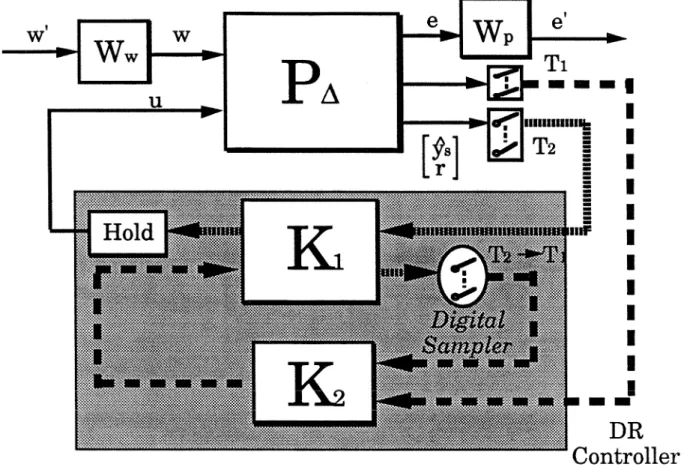
Controllers
- Thesis Overview
- Preliminaries
- Definitions, Nomenclature
- Norm of Continuous-Time Signals
- Now (Induced 12-Norm) o f Discrete-Time, Causal Convolution Opera- tors
- Definition 2.1 Structured Singular Value ( p ) Let M f C n X n and define the set A as follows
- Modelling of Systems
- Definition 2.2 Shortest Time Unit (STU)
- Definition 2.3 Basic Time Unit (BTU)
- Continuous Time
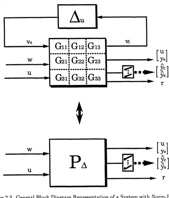
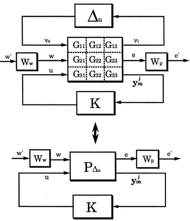
One of the main contributions of this thesis is a new Model Predictive Control technique applicable to the general inferential control problem. The frequency response matrix of the system PA I,jW belongs to the set Pu(w) where for each frequency.
2.2.2 -Discrete Time
Performance Measures
- Continuous Time
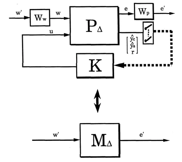
Moreover, it would provide robust performance when it meets the performance specifications despite all pre-specified mismatches between model and factory (in other words, for any system belonging to Pn). When the sampling time is chosen small in relation to the bandwidth of the closed loop, a sampled data system can be well approximated as an LTI system.
Performance Measure for LTI Systems
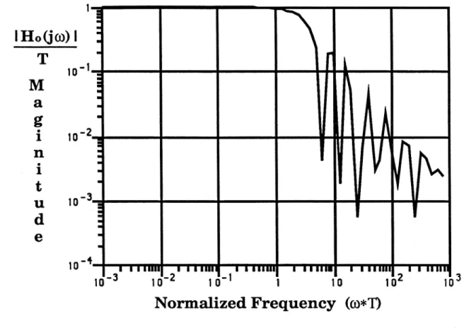
The Fourier transform of the sampled signal (ym); (expressed as impulse trains) is . The notation L{.) represents the Laplace transform. Note that the approximation of the samplers as $ does not hold outside the Nyquist band.
Frequency-Domain Performance Analysis for Multi-Rate Sampled-Data Sys- tern
Discrete Time
Analogously to the continuous-time case, one can specify performance requirements based on the H2 and H, norm of the discrete-time closed-loop operator. If the sampling time of y& is N1rS, then the fourier transform of the sampled signal is .
Description of Constraints
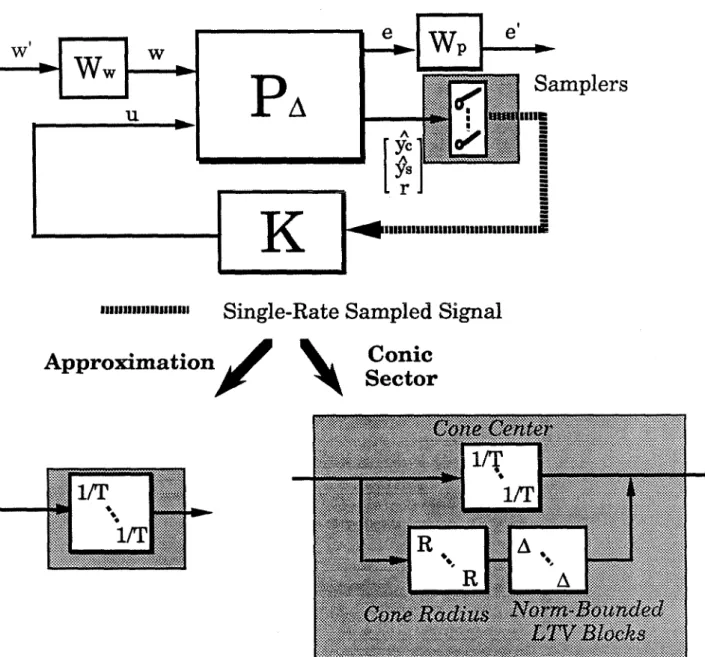
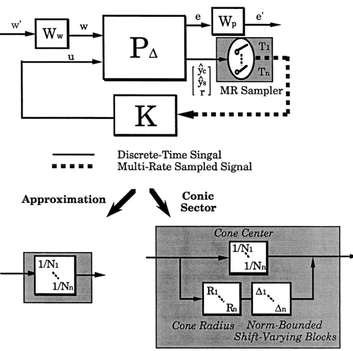
A more conservative approach is to represent these samplers as an LSI operator and a norm-limited LSV block, as in the cone-sector approach for a continuous-time system.
Chapter 3
- General Approach/Philosophy
Once the number of candidates has been reduced to a sufficiently low level, detailed analysis (such as design and simulations of the actual control system) can be performed to make the final decision. Candidate screening can be done in two steps as illustrated in Figure 3.1. The criteria that can be used to perform this design-independent screening will be referred to as "general screening tools." This screening process leaves candidates for whom a screening system leads to satisfactory results.
In the following parts of this chapter, we introduce a range of numerically efficient screening tools, both general and design-specific, that can be used to reduce the number of measurement candidates.
Design-Dependent Screening Tools I nnnnnnre
General Screening Tools
- Test Condition for Existence of a Causal Controller Achiev- ing Robust Performance
- Test Condition for Existence of a Causal Controller Achiev- ing Nominal Performance
- Test Condition for Existence of an Acausal Controller Achieving Robust Performance
First, we derive a necessary and sufficient (but not testable) condition for the existence of a controller that achieves robust performance. For stable open-loop systems, (3.21) is a necessary and sufficient condition for the existence of an acausal controller I (that satisfies the robust performance requirement. For open-loop unstable systems, (3.21) is only a necessary condition for the existence of a " acausal" controller K that achieves robust performance.
It was interpreted as a necessary and sufficient condition for the existence of an acausal controller that provides robust performance for stable open-loop systems, and as a necessary condition for unstable open-loop systems.
Design-Specific Screening Tools
- Steady-State Screening Tools
Controllers Minimizing Projection Error (LQG/MPC)
Controllers with Integral Action
Relationships with Previous Criteria
Using this method, some of the previously proposed criteria are shown to emerge naturally under specific uncertainty structures and some restrictive assumptions about performance/disturbance weights. The following lemma allows the explicit computation of the "worst case" steady-state closed-loop error [40]. In addition, let v be the input vector corresponding to the largest singular value of the matrix.
These assumptions correspond to constraining the structures of the external inputs and performance weights.
- Problem Description
- Application of Brosilow 's Criteria Brosilow's Criteria
The example will show that the new screening tools provide an effective way to analyze the sensitivity of candidate measurement sets to different uncertainty structures. Detailed information on the operating conditions and column modeling assumptions can be found in Tong & Brosilow [7]. They indicate that the above two quantities conflict as the number of measurements is varied and leave the final compromise to engineering judgment.
The original definition of the projection error is appropriate when the disturbance vector is a random variable with zero mean and an identity covariance matrix (i.e. E{d) = 0, E{ddT} = I).
Theoretical Justification of Brosilow 's Criteria
Application of General Screening Tools Physically Consistent Unstructured Ouput Uncertainty
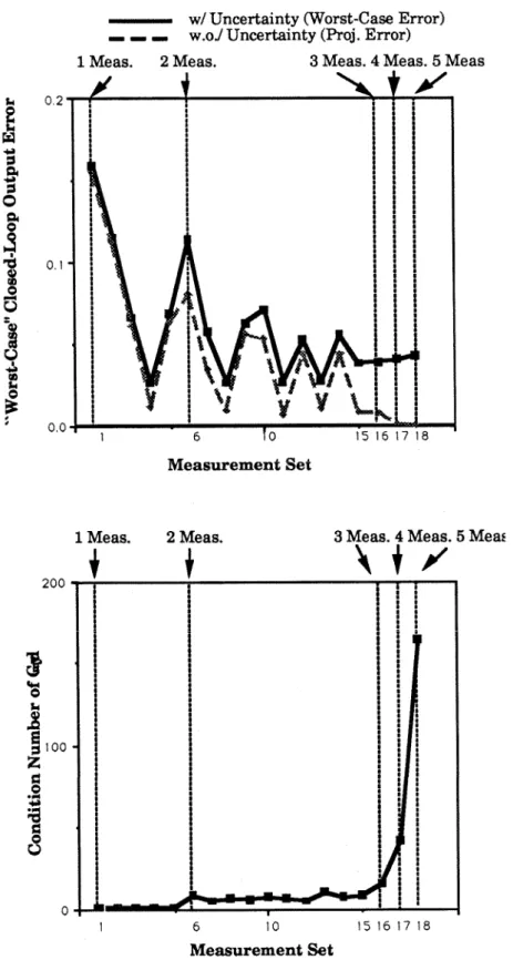
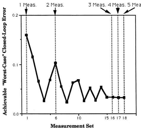
It is not our claim that the uncertainty description (3.181) is a physically meaningful one; we simply started from the uncertainty description used by Brosilow and co-workers in developing their criteria and modified it so that it became physically consistent. Because the SSV test for robust performance involves 2-block A (Asx5 and A,), General Screening Tool #3 proposed in Section 3.3 is a necessary and sufficient condition for the existence of a constant matrix K that meet a given "worst-". case" closed-loop error bound on the output. Note that, although the achievable "worst-case" error decreases as more measurements are added (consistent with our physical intuition), the "worst-case error for :y which only two measurements involve almost as low as that of five measurements measurements.
If the uncertainty description was indeed physically meaningful, the use of more than two measurements is hardly justified in this case.
Numerical Example 2: High-Purity Distillation Col- umn
It represents the measure of "worst possible" performance when the regulator is designed to provide no steady-state offsets in compositions nominally (in the absence of uncertainty and measurement error). This is evident from the plots shown in Figure 3.14(a), which represent the values for the left-hand side of inequality (3.89) when measurement error (uncompensated pressure variation) / model uncertainty is neglected. The robust performance p-plot (Figure 3.15(b)) shows that robust performance is achieved for the T7/T3.5 measurement set.
Although not shown, the SSVs for the other two candidates exceeded 1 in some frequency ranges, implying that robust performance is not achieved.
Overview
- Model Based Design
- Regression Based Design
- Use of On-Line Primary Measurements
Various modifications to the standard Least Squares method available in the literature (to overcome the collinearity problem) are discussed and their merits for estimator design are evaluated. We first discuss the design of the output estimator based on a dynamic (or static) model. In this section, we discuss the output estimator design based on the records of inputs and outputs for the estimator.
An application of the PLS method to the problem of designing a static estimator for a high purity distillation column can be found in Mejdell [45].
FPrn
Linear Quadratic Gaussian (LQG) .1 Model
- Minimization Objective
- Optimal Control Design
In the modified state space model on the other hand, modeling Ad as white noise implies that. For the modified model, the objective function weights the changes in the control inputs (Au) rather than the control inputs themselves (u). For the existence of a stabilizing solution of the above equation, we need the stability of the pair (Q,I',).
A noteworthy point is that in the above formulation the reference input vector r(k) is assumed to be a step (or integrated white noise in the stochastic framework).
Generator
Feedback
Constraint Handling: Extended Kalman Filter
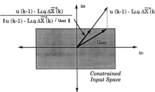
However, for multivariable systems, Autrue(k), calculated by projecting utrUe(k - . 1 ) - L L Q ~ x e ( k ) onto the limited input space of u ( k ), is generally suboptimal and can cause significant performance degradation. This is because input constraints can change the direction of the input and cause the loop gain to differ significantly from that in the absence of constraints, especially for ill-conditioned systems in combination with a directional controller.
Robust Design/Tuning
Closed-Loop Relationships
This is evident from the closed-loop relationships between Ad(k) and y,(k): yc(k) is simply expressed as white noise going through steady (closed-loop) dynamics. Note that the observer dynamics affects the closed-loop transfer function due to disturbances (Ad(k)) and measurement noise (v), but not the closed-loop transfer function from the output reference vector (Ar(k)). On the other hand, the controller dynamics affect all closed-loop transfer functions.
The function H is called the "complementary sensitivity function" and is directly related to the sensitivity and robustness of the closed-loop system.
Internal Model Control (IMC)
- Minimization Objective
- Detuning for Robustness
- State Space Formula for IMC Controller
- Constraint Handling
- Robust Desigmuning of IMC Filter
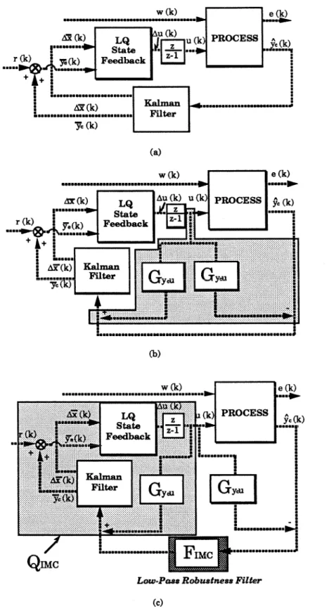
Hence, GycuQzMC represents the “ideal” complementary sensitivity function (i.e., the optimal complementary sensitivity function in the absence of measurement noise and modeling errors) that must be detuned for robustness. In this section, we briefly present a method for deriving robust performance norm bounds on desired transfer function matrices. We can parametrize the closed-loop system in terms of FIMC as shown in Figure 4.11(b) and derive the robust performance norm bound on FIMC.
A direct way to overcome this problem is to reparameterize the closed loop in terms of I - FaMc, as shown in Figure 4.11 (c) and derive the robust performance standard bound by I - FzMC.
Robust DesignJTuning Rules
Relationship with LQG and Traditional IMC
Therefore, the FzMC leading to an IMC controller equivalent to the LQG controller is simply the following diagonal first-order filter. The proposed IMC technique differs from the standard IMC technique [50] in that the IMC controllers are interpreted as state observer-based compensators and that its formulation allows the flexibility of including a nonzero input weight in the objective function. The standard IMC is developed in an input/output setting and the QIMc is calculated directly assuming a zero input weight.
The flexibility of including a non-zero input weight can be important for ill-conditioned systems for which inverse-based controllers are not desirable from a robustness point of view.
Model Predictive Control (MPC)
- Minimization Objective
- Optimal Control Design
- Constraint Handling: On-Line Quadratic Programming
- Relationship with Dynamic Matrix Control
- Algorithm
- Practical Barriers
- Constraint-Handling
In the presence of constraints described via MPC state feedback, it is replaced by an online optimizer that computes optimal control moves (without violating the given constraints) for a given number of steps ahead and performs the first move at each t = k. . In the case where disturbances and measurement noise are described as integrated (or double-integrated) white noise and white noise, respectively, use the F (or Fa) parameter for the condition estimator to adjust the closed-loop response speed. For more general perturbation cases, use the IMC estimator described in Section 4.4.3 instead of the Kalman filter to obtain state estimates, A% and A& for the prediction equation.
These assumptions, especially the first assumption, can lead to poor performance regardless of the choice of tuning parameters.
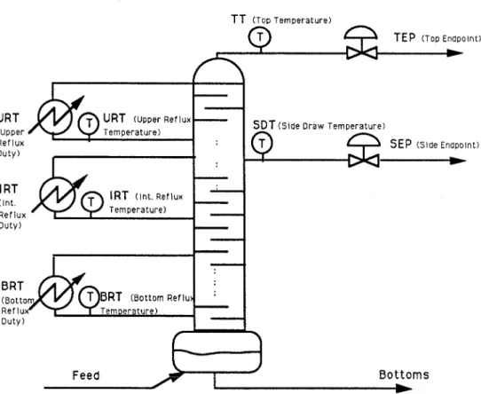
Numerical Example: Heavy Oil Fractionator
- Problem Statement
- Preliminary Analysis
- Measurement Selection and Design of an Output Estimation Based IMC Controller
We consider a simple measurement noise, which affects all temperature measurements in the same way. This is due to significant delays in measurement s; we have to use temperature measurements, which have no dead time. Since the number of disturbances we are concerned with is only two (IRD and URD), two measurements are sufficient for designing an inferential controller that gives a nominally perfect performance (i.e. in the absence of measurement uncertainty and noise).
In the next section, we investigate the feasibility of designing an IMC controller based on the output estimator that uses both the temperature and composition measurements.
Minimizing the Error Due to Uncontrollable Subspace