We also noted any chapter prerequisites as well as suggested corresponding readings from the companion text, Landscape Ecology in Theory and Practice (LETP). SEG would like to thank the late Professor Larry Harris for introducing her to the field of landscape ecology as an undergraduate student at the University of Florida.
Contents
What Is a Landscape? Basic Concepts and Tools
Fundamentals of Quantifying Landscape Pattern
Landscape Change and Disturbance
Applications for Conservation and Assessing Connectivity 12 Assessing Multi-Scale Landscape Connectivity
Ecosystem Processes and Feedbacks in Social–Ecological Landscapes
What Is a Landscape?
Basic Concepts and Tools
Introduction to Remote Sensing
OBJECTIVES
Prior to starting this lab, students are encouraged to read chapters 3 and 4 of Remote Sensing for GIS Managers by Aronoff (2005).
INTRODUCTION
Active remote sensing systems differ from passive systems in that energy is emitted from the sensor and either the return time or amount of energy reflected back by the sensor is measured. The most common active remote sensing sensors are RADAR, which transmits and detects microwave wavelengths between 1 mm and 1 m, and light detection and ranging (LIDAR), a more recent technology that transmits and receives mostly near-infrared laser pulses.
Some Remote Sensing Basics
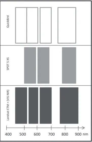
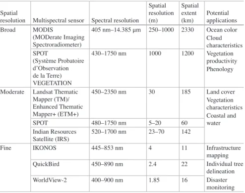
Spectral resolution can be considered in three components: the number, width, and location of the spectral wavelength bands detected by the sensor. For example, Landsat Enhanced Thematic Mapper+ (ETM+) has 7 spectral bands in the visible to infrared parts of the spectrum, while MODIS has 32 spectral bands.
EXERCISES
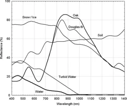
- Understanding Spectral Reponses
- Detecting the Unknown
- What Can Be Seen from Space?
- Visual Representations of Satellite Imagery
Now click the Histograms button to view the statistics for each of the color channels. Note that each band from the Vancouver Landsat scene is now loaded independently.
CONCLUSIONS
Be prepared to also submit a copy of the selected journal article when you submit your writing.
This paper provides background on conventional land cover and land use classifications for remote sensing imagery. Wulder MA, Hall RJ, Coops NC, Franklin SE (2004) High spatial resolution remotely sensed data for ecosystem characterization.
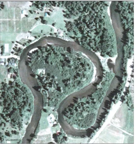
Historical Aerial Photography for Landscape Analysis
- Viewing Stereo pairs
- Seeing in Stereovision
- Exploring Manual Photointerpretation
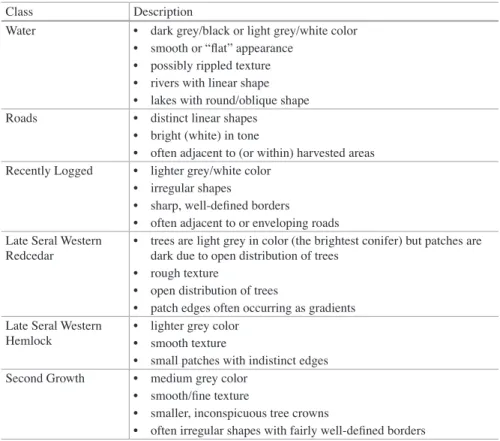
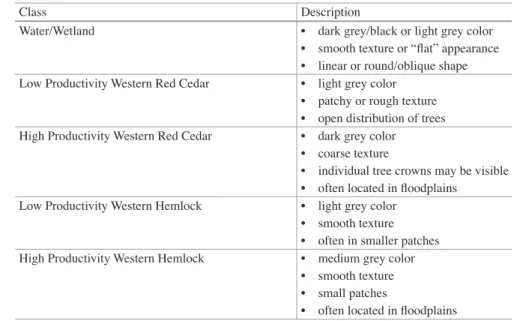
- Manual Classification of Contemporary Forests
- Reconstruction of Historical Forests
- Additional Considerations for Improving Aerial Photo Analysis
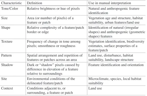
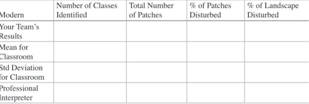
Using the same general approach as for the modern recordings, fill in the required information for your team's results in Table 2.5 based on your interpretation of the historical recordings. Q7 Which of the eight characteristics of manual interpreting (Table 2.1) were most useful in guiding your interpretation.
Impact of Errors
Uncertainty in Classification
Q12 Misclassification rates for forest inventories derived from manual interpretation of aerial photography can be as high as 60% (Thompson et al. 2007).
Historic Harvest Patterns and Topography
Benefits of Terrain
Forest Productivity in Historical Forests
Are you more or less sure of your results and interpretation after recording the uncertainty maps.
SYNTHE SIS
Morgan JL, Gergel SE, Coops NC (2010) Aerial photography: a rapidly evolving tool for ecological management. Excellent example of the global utility of aerial photography for assessing landscape change along with explaining the sometimes arduous process of building an archive.
Citizen Science for Assessing Landscape Change
Working independently, you will assess land use/land cover (LU/LC) change over the past 50 years in the Montérégie region of Quebec, Canada. In Part 1, you'll get to know the region by exploring aerial photos and land cover classifications from previous decades using Google Earth.
Fundamentals of Quantifying Landscape Pattern
First, Chapter 4 introduces you to pattern analysis using FRAGSTATS software, the longtime workhorse of pattern analysis. Exposure to QRule software helps underscore the impact of different patch definition rules on landscape metrics and the appropriate use of spatially neutral landscape expectations.
Understanding Landscape Metrics
Metrics of Landscape Composition
Information-theoretic metrics were first developed by Shannon (1948) and first applied to landscape analysis by Romme (1982) to describe changes in the area occupied by forests of different successive stages over time in a watershed in Yellowstone National Park, Wyoming. The unnormalized forms of these measures are very sensitive to the number of cover types S in the landscapes, and therefore comparisons between landscapes that differed in S were problematic.
CALCULATIONS
D values close to 1 indicate a landscape dominated by one or a few cover types, while values close to 0 indicate that the proportions of each cover type are nearly equal. Values for SHEI range between 0 and 1; values close to 1 indicate that the proportions of each cover type are nearly equal; values close to 0 indicate a landscape dominated by one or a few cover types.
Metrics of Landscape Composition in an Early-Settlement Landscape
- Calculate Dominance for the post-settlement landscape and record it in Table 4.2
- Calculate Shannon Evenness for the post-settlement landscape and record it in Table 4.2
- Calculate Dominance for the early-settlement landscape and record in Table 4.1
- Calculate Shannon Evenness for the early-settlement landscape and record in Table 4.1
If you were doing an analysis of a real landscape, would you report both D and SHEI. Q3 Use your calculator to perform some additional calculations of D using the ratios listed in Table 4.3.
Metrics of Landscape Composition in a Post-settlement Landscape
Q1 How would you interpret/describe the changes in this landscape between the two time periods. Question 6 Given your interpretation of the data in Table 4.3, what other types of information and/or metrics would be needed to distinguish between these landscapes.
SYNTHESIS QUESTIONS
Metrics of Spatial Configuration
- neighbor rule specifies that two grid cells of the same cover type are to be considered as part of the same patch if they are adjacent or diagonal neighbors
For example, the total linear edge in a landscape can be divided by the landscape area to provide a single estimate of edge: area, or edge density. If the actual boundaries of the landscape image are considered edges, it affects both edge counts and edge:area ratios.
Metrics of Spatial Configuration in an Early-Settlement Landscape
Using the results from Calculation 9, compute the edge:area ratio for each cover type and enter into Table 4.5
Adjacency probability (qi, j) is the probability that a grid cell of cover type i is adjacent to a cell of cover type j. Values along the diagonals of the Q matrix (the qi,i values) are useful measures of the degree of clumping found within each coating type.
Metrics of Spatial Configuration in an Early-Settlement Landscape (Continued)
To begin calculating Contagion, use Figure 4.2 to calculate the proportions occupied by each of the three land cover types in the subset of the early-
In particular, diagonal elements, representing adjacent cells of the same type, were counted only once. So that each proximity is counted equally, double the values of the diagonal elements of Table 4.7 and enter them into Table 4.8, the N matrix.
Use the values of the N matrix (Table 4.8) to compute the elements of the Q matrix (Table 4.9)
Calculate the Contagion value for the subset of the early- settlement landscape using the elements of the Q matrix
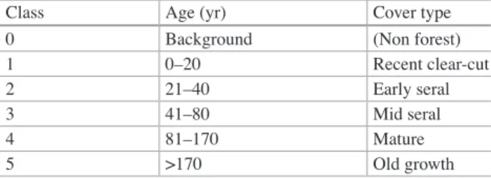
If you could divide the landscape into tiles small enough to calculate the contamination in each tile, you could combine the results in each tile to show the full extent of the contamination. The map of the first period contains five cover types; the map from the second time period contains seven cover types because 'forest' has been mapped in more detail in t2 - as deciduous, coniferous and mixed forest.
SYNTHESIS
- Using Fragstats for Automated Landscape Metric Calculation for the Early- and Post-settlement Landscapes
- Early-Settlement Landscape with the 4-Neighbor Rule
- Early-Settlement Landscape with the 8-Neighbor Rule
- Post-settlement Landscape with the 4-Neighbor Rule
- Post-settlement Landscape with the 8-Neighbor Rule
- Automated Landscape Metric Calculation for Real Landscapes and Interpretation of Multiple Metrics
- Madison, Wisconsin, USA
- Understanding Landscape Change Through Metrics
Calculate at least the following metrics with Fragstats for each of the maps described below. In this section, you will explore some of the challenges of using landscape metrics to assess landscape change through time.
Scale Detection Using Semivariograms and Autocorrelograms
On the other hand, two locations that are at different latitudes will have different temperatures, and the amount of temperature difference will be positively (and gradually) related to the difference in latitude. However, two locations several feet apart may or may not have similar amounts of sunshine - much depends on the size and spacing of the trees.
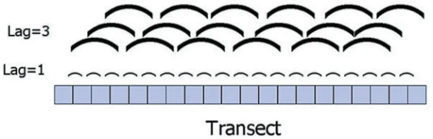
Variography
It is possible (and indeed likely) that variation in nature increases continuously as a function of scale. Since very few pairs of points represent very long distances, it is usually inadvisable to plot γ(h) for large h.
Autocorrelation
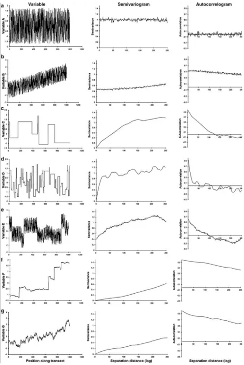
Note that only three of the variables (C, D, and E) have semivariograms that remotely resemble those in Figure 5.2. Note that the F variable has very little fine-scale noise, and therefore has a negligible nugget.
Comparing Autocorrelation to Semivariance
Data Collection
Select a field area in which the maximum vegetation height is about 2.5 m or less, and in which it is possible to establish a 200 m transect. If you don't have the luxury of a large enough place in the field, it is possible to perform this exercise with smaller connected squares.
Data Analysis
It is of course possible to put the number 198 in the denominator, but writing out the formula often helps with troubleshooting. Thus, the formula will return the semivariance for the lag specified in the same row in column C.
Results
This is similar to the observation that variance does not fully describe the statistical distribution of data (e.g. whether it is normally distributed), and that the correlation coefficient does not fully describe the nature of the relationship between two variables (e.g. a non-linear relationship). What do you expect will happen to the semi-variogram if you reduce the size of the square.
OPTIONAL EXERCISES
Correlation and Variation
The provided data sets (on the example data sets page in the spreadsheet accompanying this lab) can be pasted blank into the data column (column B) in the ready-to-go worksheet, and the semivariograms and autocorrelograms will be recalculated automatically (Note however that you may need to change the Y-axis scale on the graphs). Choose two or three of the variables and describe what natural phenomena can lead to those patterns.
Variography and Fractals
Variography using R
FURTHER STUDY
The most common product of kriging is a map (usually a contour map) of the variable of interest. As Wagner (2003) elegantly illustrates, distance decay in species distributions scales up to distance decay in species richness, one of the root causes of the species-area relationship (Palmer and White 1994).
Characterizing Categorical Map Patterns Using Neutral Landscape Models
Simple Random Map(s) Analyzed with Three Different Neighborhood Rules
If tail, then habitat type is equal to 1. Analyze the map by coloring in all places with habitat type = 1. Count the total number of cells colored, the total amount of edge, the number of clusters as determined by the nearest neighbor rule contiguous , and the size of the largest group. Using the nearest neighbor rule, recalculate the number of clusters and the size of the largest cluster.
Using Q RULE to Generate and Analyze Neutral Landscape Models
Random Maps and Critical Thresholds
Repeat the above process described in steps 2-4, run QRULE separately for each script file and then rename the log files and patch_cfd.dat and statistics. Q4 Were the resulting fractions of each land cover type in the results (see the logs) equal to what was specified in the script files.
Spatial Contagion
Open this script file and change the neighborhood line to the one assigned to your last name in the exercise above. What differences do you see in the cumulative frequency distributions (CFDs) for the random and multifractal maps.
Neutral Models and Actual Landscapes
Which differences are statistically significant (ie, the metric value for the actual landscape lies outside the range in the neutral landscape model) or would be ecologically significant. The existence of critical thresholds in landscape connectivity was also explored in the analysis of neutral landscapes.
What Constitutes a Significant Difference in Landscape Pattern?
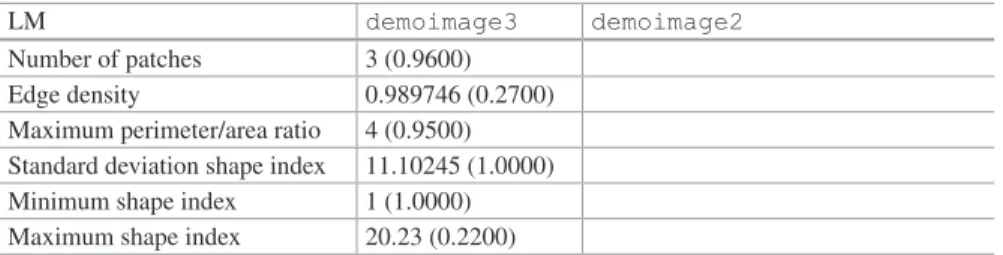
Analysis of a Single Landscape
The probabilities above indicate how likely the observed map LM is relative to the simulated values (the null, empirical distribution). Thus, P = 0.9600 that the observed LM value for the map is less than what would be expected from the empirical distribution (because there are many more simulated landscapes that had higher values).
Comparing Two Different Landscapes
The importance of each class-level metric can be assessed by calculating its probability (ie, how many times the observed class-level metric is greater or less than the expected metric under the empirical null distribution based on 100 replications ). Assess whether there is a significant difference for each grade-level metric for each observed landscape and interpret the results to determine whether the confidence intervals of each metric overlap.
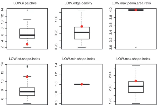
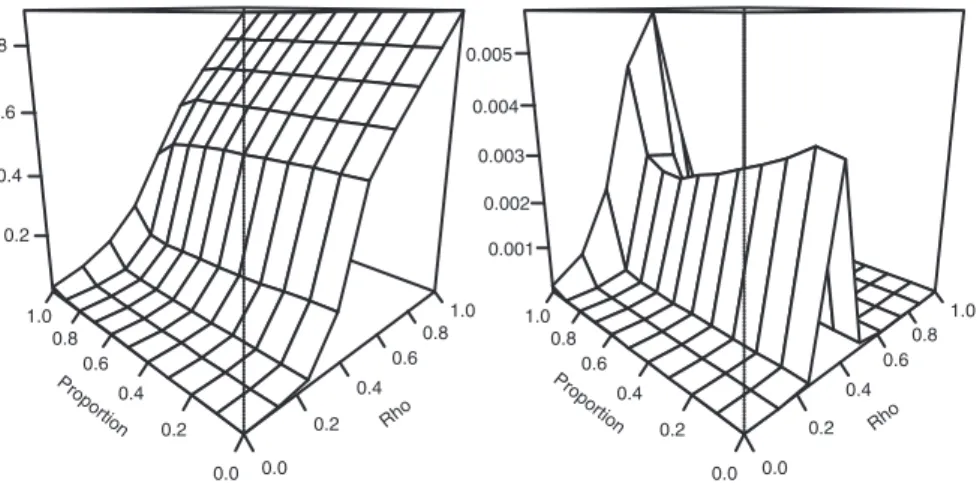
Determine a Landscape’s Position Within the Distribution of Possible Class-Level Metric Values
The objective of this third exercise is to determine where the observed landscape exists within the class-level metric space based on its proportion and estimated degree of spatial autocorrelation. Include box plots for step 1 at the observed proportion level and the spatial autocorrelation (ρW) axis on the surface to show variability (set cross=TRUE for this).
APPENDIX A. EXPLANATION OF WHITTLE’S ALGORITHM (WHITTLE 1954)
Riitters KH, O'Neill RV, Hunsaker CT et al (1995) A factor analysis of landscape pattern and structure metrics. This cornerstone paper summarizes the redundancies present among many landscape pattern metrics and proposes new composite variables to characterize landscape patterns.
Landscape Change and Disturbance
Introduction to Markov Models
The elements, nij, of the count matrix count the number of cells that have changed from type i to type j during a time interval. The elements, pij, of the transition matrix P summarize the proportion of cells of each cover type that changed to another cover type during that time interval.
Markov Models
The stationary or equilibrium state of the system is given by the eigenvector of the transition matrix; thus there is a closed form model solution. The thickness of the arrows indicates the extent of transition stages between different types of coatings (arrows for self-interchangeability are not shown).
Modeling Landscape Change in the Pacific Northwest, USA
- Model Development
- Model Verification Via Matrix Projection By Hand
- Matrix Projection Using the Program M ARKOV
- Model Validation
Note the indices to ensure that the appropriate elements are used: internal indices must always match (ie the index on x must match the first index on p). When you are asked for the number of patch types, this refers to the number of cover types in the model.
Further Considerations in Modeling Landscape Change
Note that in the limit, the average of a large number of stochastic simulations will be a map of the transition probabilities themselves. These cases would lead to higher-order Markov models (eg, in a second-order model, one would need to know the state of the system at time t and t−1 to predict its state at time t + 1).
WRITE-UP
Acevedo MF, Urban DL, Shugart HH (1996) Models of forest dynamics based on the roles of tree species. Hong SH, Mladenoff DJ (1999a) Spatial explicit and stochastic simulation of fire disturbance and succession in forest landscapes.
Simulating Management Actions and Their Effects on Forest Landscape Pattern
The model allows you to change the size of timber harvest openings, the total area harvested, and the spatial distribution of harvested areas (whether harvests will be clumped or spread). You will determine how different harvesting regimes affect the amount of forest interior, amount of forest edge and the average patch size of forests.
INTRODUCTION Simulation Modeling
This use allows insight into the implications of the view of reality that is formalized in the model. The model allows changing the size of the cut openings, the total cut area and the spatial distribution of the cut areas (whether the cuttings will be clustered or scattered).
Change in Spatial Pattern
These models differ in the required input data and the complexity of the scenarios they can simulate. The amount of interior present is quite sensitive to the width of the edge buffer under certain forest opening patterns, as you will find.
The HARVEST L ITE Model
This is the percentage of the forested area in the input map that is cut by the model every decade. It is the average size (ha) of forest patches, where patches are defined as contiguous cells of the same forest age.
Instructions for Using the HARVEST L ITE Model
- Effects of Mean Harvest Size on Forest Pattern
- Effects of Percent of Forest Cut Each Decade on Forest Pattern
- Effects of Spatial Dispersion on Forest Pattern
- Effects of Edge-Buffer Width and Opening Persistence Time on Forest Pattern
Calculate the amount of forest interior using an edge-buffer distance of 180 m and an opening period of 20 years. Calculate the amount of forest interior using an edge-buffer distance of 180 m and an opening period of 20 years.
Regional and Continental-Scale Perspectives on Landscape Pattern
- Estimating Landscape Metrics by Eye
- Visual inspection
- Ranking using metrics
- Metric Finder: Relating Visual Assessments to Landscape Metrics
- Labeling Landscapes Using Metrics of Proportion
- Metrics of Proportion for Rare Classes
- Labeling Landscapes Using Metrics of Configuration
- Grouping Landscapes with Metric Finder
- Exploring Variation in Landscape Metric Values Across a Region
- Using Metaland to Select Landscapes with Geographic Criteria
- Estimating Histograms and Testing Expectations
- Histograms of Other Land-Cover Proportions
- Selecting Study Landscapes Along Gradients
- Controlling for Proportion and Total Edge
- Synthesis
- Identifying Landscapes Along Two Gradients
- Complementary Work with Metric Finder and Metaland Metric Finder is linked to Metaland, and this linkage allows you to select a subset
- Designing Regional Comparisons
When differentiating the landscapes for this exercise, pay attention to the area of the Metric Finder interface that shows the clustering assignments projected across all the landscapes in the set. Q7 How successful is the mapping of the entire set of landscapes against your defined selection criteria.

Using Spatial Statistics and Landscape Metrics to Compare Disturbance Mosaics
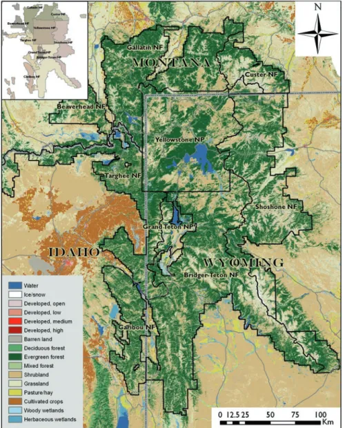
In this lab, students will compare the spatial patterns generated by three different types of disturbance using spatial statistics and landscape metrics and then compare the interpretations that emerge from these complementary approaches. Determine and compare landscape patterns created by fire, insect outbreaks, and clear-harvest in forested landscapes of Greater Yellowstone (Wyoming, USA) using spatial statistics applied to continuous measures of disturbance severity;.
Study Area and Disturbances
- Using Spatial Statistics to Compare Mosaics Generated by Different Disturbances
- Describing Disturbance Patterns Qualitatively
- Quantifying Disturbance Patterns Using Spatial Statistics Next, describe the spatial patterns of each disturbance type using variograms and
- Understanding Differences Among Theoretical Models of Semivariance
- Analyzing Fire Patterns Using Landscape Metrics and Spatial Statistics
- Selecting Landscape Metrics
- Quantifying Fire Patterns Using FRAGSTATS
- Using Spatial Statistics and Landscape Metrics to Compare Disturbance Mosaics
Q1 In your own words, qualitatively describe the spatial patterns of the three types of disturbance (Figure 11.2). For each of the ten landscapes (2 thresholds × 5 replicates = 10 landscapes), you will use FRAGSTATS to characterize the spatial patterns of the burned landscapes.
Applications for Conservation and Assessing Connectivity
Assessing Multi-Scale Landscape Connectivity Using Network Analysis
You then calculate and compare two simple metrics of landscape connectivity for these two networks. In Part 2, you will examine the impacts of landscape connectivity on protected areas in the Willamette Valley ecoregion of the United States in a more realistic example.
Landscape Connectivity