Searching for Gravitational Waves from Compact Binary Coalescences and Stochastic Backgrounds in the

Introduction: The Dawn of Gravitational-wave Science

A Brief History of the Hunt for Gravitational Waves

Even in the 1960s, the idea of ​​interferometric GW detection was independently pursued by several researchers. On the theoretical front, Kip Throne led a group at Caltech to study the theory of GWs and their astrophysical sources and later noise in GW interferometers in the 1970s.

Outline of Chapters

The inherent condition number of the matrix, that is, the ratio between the minimum and maximum eigenvalues, depends on the spectral shape. Accessibility from the stochastic gravitational wave background of magnetars to the interferometric gravitational wave detectors”.

Introduction to Gravitational Waves and LIGO

Gravitational Waves in General Relativity

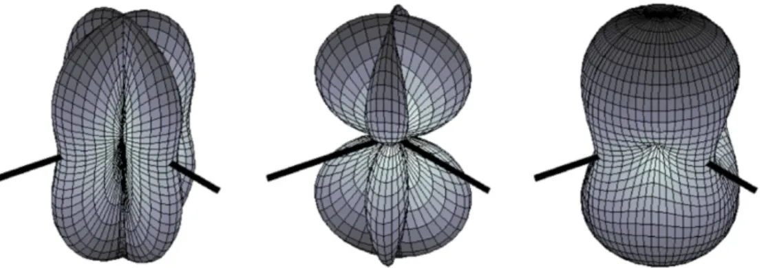
The effect of the passage of a GW is thus to cause a tidal deformation of objects transverse to the wave's direction of propagation. Provided that the size of the source is much smaller than its distance to the observer. 2.36).

Figure 2.1: The effect of a monochromatic gravitational wave with angular fre- fre-quency 𝜔 = 2 𝜋 / 𝑇 propagating perpendicular to the plane of a circular ring of test particles

Sources of Gravitational Waves

Kepler's third law relates the orbital period𝑃with the total mass 𝑀 and the orbital separation𝑎, 𝑃2 ∝ 𝑀−1𝑎3. For space-based interferometers, the targets are GW sources in the mHz and deci-Hz range.

Figure 2.2: Sources associated with each gravitational wave frequency band and the corresponding types of detectors required for detection [38]

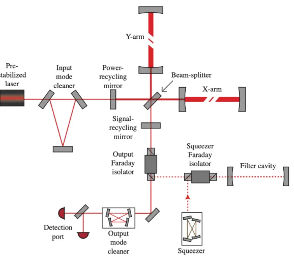
Advanced LIGO Detectors

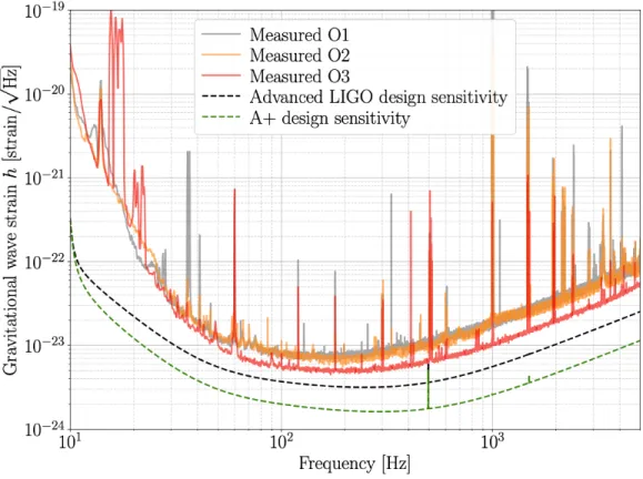
Compression further reduces phase quadrature noise at the expense of larger amplitude fluctuations, allowing for more accurate photon arrival time measurements. In Figure 2.4, we show representative GW spectra of the sensitivity of the Advanced LIGO Hanford detector in the first three observing runs (O1, O2 and O3), as well as the Advanced LIGO design curve planned for the fourth observing run (O4) and the target curve of the future upgrade, A+, for the fifth observation (O5).

Figure 2.3: A simplified optical layout of an Advanced LIGO detector planned for the fourth observing run (O4)

Overview of LIGO Science

In the presence of only Gaussian stationary noise, the statistical properties of the detector noise 𝑛(𝑡) are well characterized by the one-sided power spectral density (PSD) written as. Gravitational wave geodesy: a new tool for validating the detection of the stochastic gravitational wave background”.

Compact Binary Coalescences

Astrophysical Processes

In a binary, the Roche radius of the primary star's critical gravitational potential writes approximately [132]. This quadruple moment causes loss of the binary's orbital energy, with the precise dissipation process and rate depending on the stellar structure [ 134 , 135 ].

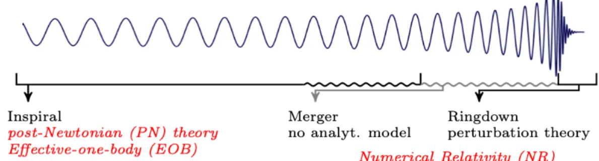
Gravitational Waveforms

On the basis of the −2 spin-weighted spherical harmonics −2𝑌𝑙 𝑚(𝜃 , 𝜙), is the multipole decomposition of the strain. In the spectral model-dependent broadband searches, we find no excess signals on top of the detector noise.

Figure 3.1: The inspiral, merger and ringdown stages of the GW signal from a non- non-spinning BBH merger as a function of time

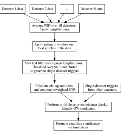
The PyCBC Search Pipeline for Gravitational Waves from Com-

Matched-filter Search Pipeline

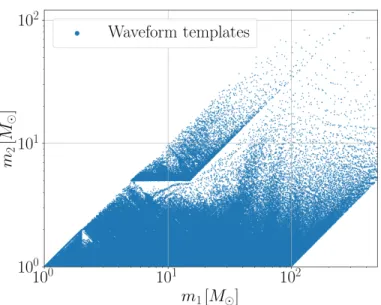
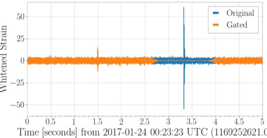
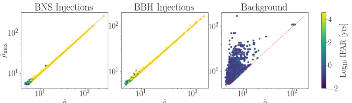
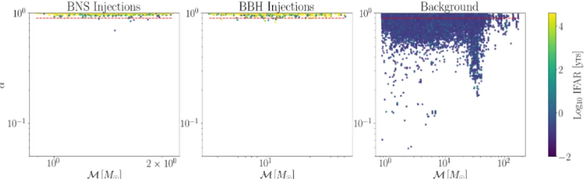
The density of templates across the bench is determined by the PSD of the detectors. Another method to handle errors is by "painting in" the identified bad data segments so that the twice whitened data is zero at bad times [206]. 0 is the central frequency and time of the sine Gaussian, respectively, 𝑄is the quality factor currently set to 20, 𝐴 is the amplitude set to 1, and𝜙. The sine-Gaussian 𝜒2 discriminator is most effective in preventing errors from causing high-mass templates with final frequencies of ∼100 Hz or less, increasing the search sensitivity for high-mass BBHs.

4.19) Noise Model – The simultaneous noise rate density is estimated by fitting the distribution of triggers above a realigned SNR threshold in the individual detectors and combining the trigger rates for different detector combinations.

Figure 4.1: Antenna patterns of a LIGO GW detector in the small-antenna limit ( 𝐿 𝑐 / 𝑓

PyCBC Live: A Real-time Search

A GW detector network is diffraction limited, i.e. the resolution and thus the point spread function inherently depends on the frequency of the source. We also place constraints on the spectral shape of the SGWB using the spectral model-independent method described in Section 7.2. Sensitivity of the Laser Interferometer Gravitational Wave Observatory to a stochastic background and its dependence on the detector orientations”.

Results of the PyCBC Search across LIGO–Virgo’s First Three

Gravitational-wave Transient Catalogs

During O1 and O2, the BNS inspiration range extends from 60 Mpc to 80 Mpc for LIGO Hanford and from 60 Mpc to 100 Mpc for LIGO Livingston. Thanks to several improvements during the commissioning period before the start of O3a, all three detectors improved their sensitivity significantly, with the average BNS inspiration interval reaching 108 Mpc for LIGO Hanford, 135 Mpc for LIGO Livingston and 45 Mpc for Virgo [228] . Among the 39 reported candidates, 27 were detected by PyCBC, less than the number of 36 for GstLAL, mainly due to the exclusion of the Virgo data.

Compared to O3a, the average BNS inspiration intervals are 115 Mpc for LIGO Hanford, 133 Mpc for LIGO Livingston, and 51 Mpc for Virgo.

Figure 5.1: Masses of BHs and NSs in the stellar graveyard detected through GWs and EM waves

Exceptional Gravitational-wave Events

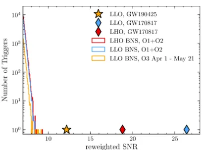
GW190412 is unique in that it was the first fusion detected with indisputably significant unequal masses [256]. GW190425 was first identified on April 25, 2019 as a single-detector event in the LIGO Livingston detector by the low-latency GstLAL pipeline with a matched-filter SNR of 12.9 [260]. No evidence of tidal effects or spin-induced quadruple effects in the signal has been found, and no EM counterpart has been identified.

For both events, no evidence of tidal effects or spin-induced fourfold effects was found in the signal, and no EM counterpart has been identified.

Figure 5.3: Histogram of reweighted SNRs for single-detector triggers in the BNS region

Conclusions

Stochastic Gravitational-wave Backgrounds

Properties of Stochastic Backgrounds

GWi is the GW energy density and 𝜌𝑐 is the critical energy density required to close the universe today. Conceptually, ΩGW(𝑓) (d𝑓/𝑓) is the ratio of the GW energy density to the total energy density required to close the universe today in a small frequency range from 𝑓 to 𝑓 +d𝑓. For an isotropic background, we can relate the GW energy density spectrumΩGW(𝑓) and the strain power density spectrum𝑆ℎ(𝑓) with.

Assuming that an SGWB is Gaussian, stationary and unpolarized, the statistical properties of the isotropic background are completely specified by its energy density spectrumΩGW(𝑓).

Sources of Stochastic Backgrounds

The total energy density in GW normalized by the critical energy density is therefore ΩGW=. 6.16). We can then compareΩGW to other forms of energy density in the Universe: Ω𝑅, radiation including photons and relativistic neutrinos;Ω𝑀, matter including baryons and cold dark matter;Ω𝑘, spatial curvature; andΩΛ, vacuum energy. The energy density spectra due to CBCs and the comparison with the current and future sensitivity of the detector are shown in Fig.6.2.

The superposition of these GW bursts from cosmic strings or cosmic superstrings over the history of the universe creates an SGWB [268,269].

Figure 6.1: The landscape of potential SGWB signals and various current observa- observa-tional constraints across the frequency spectrum, taken from [69]

Detection Methods

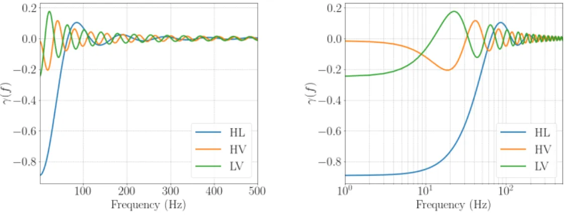
When detector noise is uncorrelated within the baseline, the expected value of the cross-correlation between the strain in detector 1 is 𝑠. However, there is a type of noise, the Schumann magnetic resonances, caused by the Earth's EM field, which can mimic a correlated SGWB in the detectors. Fig.6.3 shows the normalized ORFs for LIGO Hanford – LIGO Livingston1 (HL), LIGO Hanford – Virgo (HV), and LIGO Livingston – Virgo (LV) baselines in the small antenna limit (𝐿 𝑐/𝑓 . GW), down to 500 Hz.

For the spectral index 𝛼, Ω𝛼 is the normalized GW energy density at the reference frequency 𝑓. ref, usually selected in the most sensitive area of ​​analysis.

Figure 6.3: Normalized overlap reduction functions (ORFs) 𝛾 ( 𝑓 ) for constitut- constitut-ing baselines HL, HV and LV in the HLV detector network in the small-antenna limit ( 𝐿 𝑐 / 𝑓

Current Observational Constraints from LIGO–VIRGO–KAGRA

We also show the upper bounds of the angular power spectrum𝐶𝑙's for SGWB obtained via Eq. At the time of the project, the development of a robust KF in TCS was still at an early stage. GWTC-2: Compact Binary Coalescences Observed by LIGO and Virgo During the First Half of the Third Observing Run”.

Table 6.2: 95% confidence-level upper limits on the normalized GW energy density, normalized GW energy density spectrum and GW energy flux using combined data from LIGO–Virgo’s first three observing runs [292, 293]

Model-independent Search for Anisotropies in Stochastic Gravitational-

SGWB Mapping

2(𝑡;Θ𝑝)𝑒🝑 air discretized in the pixel domain, that is, it is the direction pointing to the center of the pixel𝑝. Due to limited coverage of the sky, signals from point sources spread to other locations on the sky. To use the deconvolution in Eq. 7.16), we need to invert the Fisher matrix, which is typically singular due to the uneven sampling of the sky.

Analogous to the approach in the CMB experiments, we construct unbiased estimators of the square of the angular power ˆ𝐶𝑙 in the spherical harmonic basis z.

Figure 7.1: Point spread functions Γ 𝜂𝜂 0 for the HLV detector network in its O3 sensitivity, assuming a flat strain spectrum for point sources

Spectral Shape: Model-independent Approach

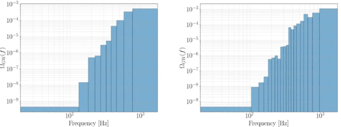
The optimal state number of the Fisher matrix for each band would ideally be determined independently using the method presented in Section 7.1 with a monopole simulation in that band. Assuming an angle-independent spectral shape and with the Fisher matrix properly conditioned, estimated GW energy densities in each frequency band will trace the strain-force spectral dependence. In the spectral-model-independent method, a single angular resolution does not accommodate all frequency bands due to different diffraction limits defined via Eq.

Fixing an angular resolution across all bands over-resolves lower frequencies and therefore degrades Fisher matrix conditioning and under-resolves higher frequencies and thus loses achievable SNRs.

Simulations

Upper Limits on Anisotropic Backgrounds through LIGO–

Spectral-model-dependent, Broadband Limits

To confirm this, we calculate p-values ​​from the distributions of the SNR maps; these are also listed in Table 8.1. These are roughly consistent with the results of the anisotropic LVK search [293], given that the regularization is performed very differently, so the dispersion over the ℓ modes appears different in the two upper limits. Our choice of the largest ℓmode included here is dictated by our pixel resolution, along with the expected angular resolution of this search style discussed in [293] .

The relationship betweenℓmode and number of pixels needed to resolve it, expressed in terms of the HEALPix 𝑁.

Figure 8.1: Clean maps, SNR maps, Ω GW upper limit maps, noise maps and SNR histograms for results integrated over a broadband of frequencies between 20 and 1726 Hz at a reference frequency of 𝑓

Spectral-model-independent, Narrowband Limits

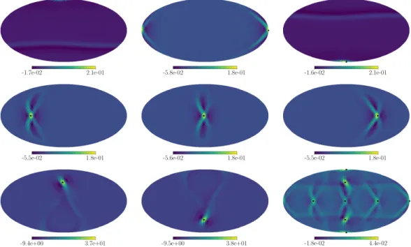
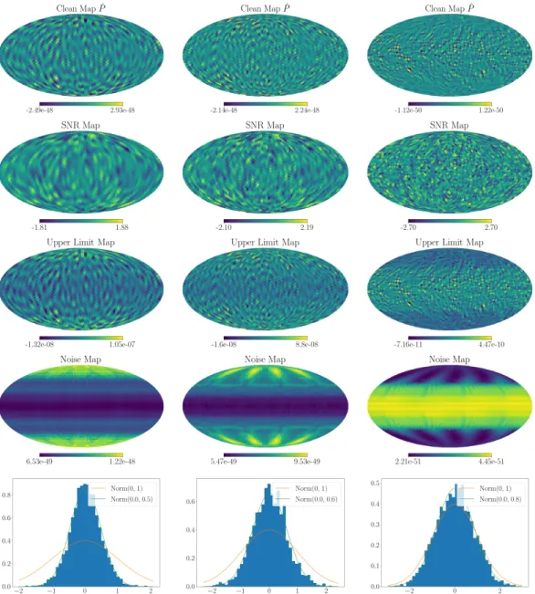
We observed a deviation for ℓ =6 in the case of 𝛼=3: this is currently under investigation and is believed to be due to the noise fluctuation that makes the point value 𝐶. We also show the clean maps, SNR maps, and noise maps for the three narrowband analyzes at low, mid, and high frequencies of the 10-band example in Fig. We observe that changes in the extent of the structures are evident as the frequencies increase and our method selects the resolution of each band accordingly, as shown in Figure 8.4.

Figure 8.3: 95% upper limits on the energy densities in distinct frequency bands used in the spectral-model-independent spectral analysis

Discussion and Future Work

Advanced LIGO Detector Commissioning for LIGO–Virgo’s

Implementation of a Real-time Kalman Filter in the LIGO Thermal

Absorption of laser power in the test masses produces temperature gradients over the entire volume of the test masses and forms thermal lenses. A number of analytical models of the temperature fields and thermo-optical aberrations in the test masses have been developed [381, 382]. Spherical power, denoted by 𝑆, is the spherical component of the optical aberration𝜓, and is inversely proportional to the radius of curvature.

Finally, we get a representation of the state space, which has the form of Eq. where Δ𝑡 is the KF sampling period.

Figure 9.2: A schematic of the Advanced LIGO Thermal Compensation System.

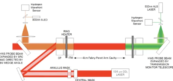
Calibration of Subsystem Cavity Lengths

Summary and Outlook

Summary of the Previous Chapters

Since then, through the end of LIGO-Virgo's third round of observations, the LIGO Scientific, VIRGO, and KAGRA collaboration has cataloged dozens of GW signals from compact binary fusions, bringing the total number of GW events to 90 [6]. They even provide a glimpse into the earliest moments of the Big Bang and provide a standard way of measuring the expansion history of the Universe [29]. Leading up to the sensing aspect of GWs, we also introduced the advanced LIGO detectors for measuring the stretching and squeezing of spacetime and the scientific values ​​of such efforts in fundamental physics, astrophysics and cosmology.

In addition to maximum likelihood map modeling, we have also implemented a model-independent method to investigate the spectral shape of stochastic backgrounds.

Outlook