Sixth, I would like to thank my colleagues at Caltech, both inside and outside Vi-. I would also like to thank Marco Andreetto and Ahmed Elbanna for helpful and insightful discussions.
Introduction
Introduction
In this chapter, we provide an overview of the problem of image retrieval, which is discussed in the thesis. Finally, Section 2.5 describes the full representation approach, followed by the bag-of-words approach in Section 2.6.
Image Search Problem
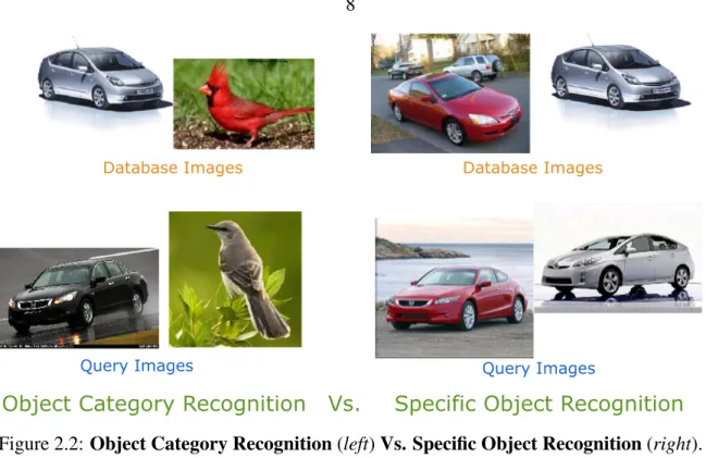
The system searches the database and responds with the identity of the search object, along with some useful information. The systems we are interested in must return the identity of the specific object shown in the query image.
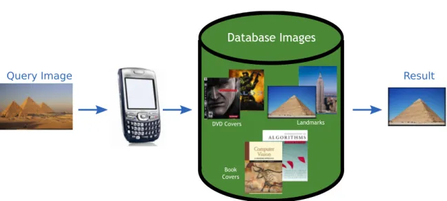
Image Representation
Local features: where the image is represented by a set of local feature descriptors extracted from a set of regions around the image. In this thesis we focus on using local features for large-scale image search, as they have much higher performance than global features provide.
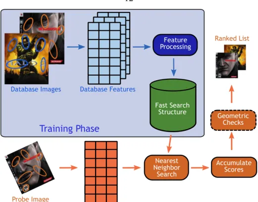
Basic Image Search Algorithm
In the data structure, each attribute g(fi j) is associated with one (or more) database images that contain that attribute. In the training phase, local features are extracted from the database images, optionally processed, and then inserted into a fast search data structure.
Full Representation (FR) Image Search
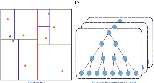
- Kd-Trees (Kdt)
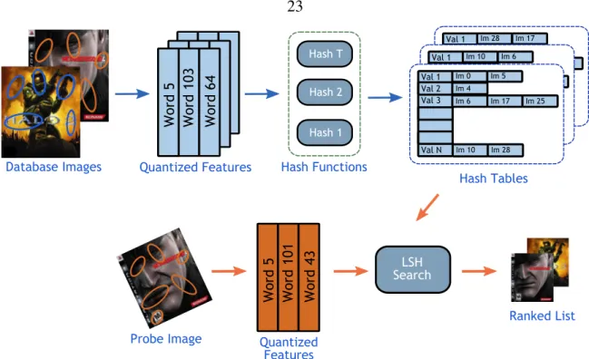
- Locality Sensitive Hashing (LSH)
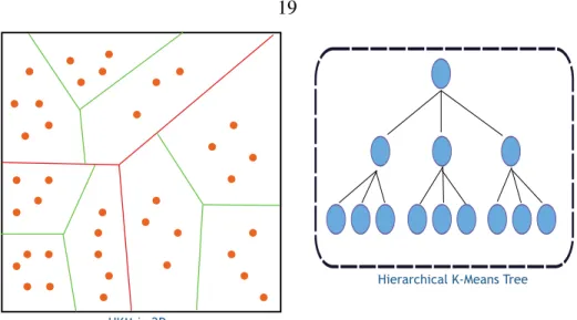
- Hierarchical K-Means (HKM)
The nearest-neighbor search is done indirectly via vector quantization of the feature space, as opposed to directly searching the feature space as in FR search (see Figure 2.6). However, for a fixed number of features, this reduces the runtime as it creates more leaf nodes in the bottom of the tree.
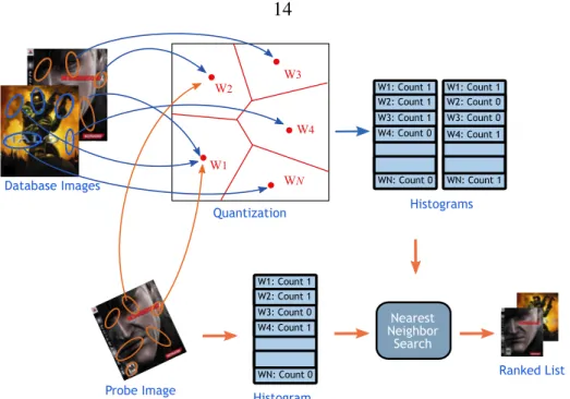
Bag of Words (BoW) Image Search
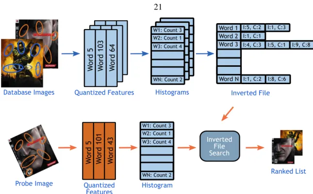
- Inverted File (IF)
- Min-Hash (MH)
Using fewer sight words usually results in poorer performance, while using a much larger number of sight words also hurts performance. The hash function is defined ash(b) =minπ(b)whereπ is a random permutation of the numbers{1, ..,W}, where W is the number of words in the dictionary.
Summary
In general, the larger the dictionary, the better the performance and the faster the actual search, because the number of overlapping images is smaller. In the next chapter we will detail the theoretical analysis of the properties of these methods and how they scale with very large numbers of images.
Introduction
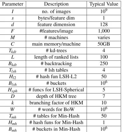
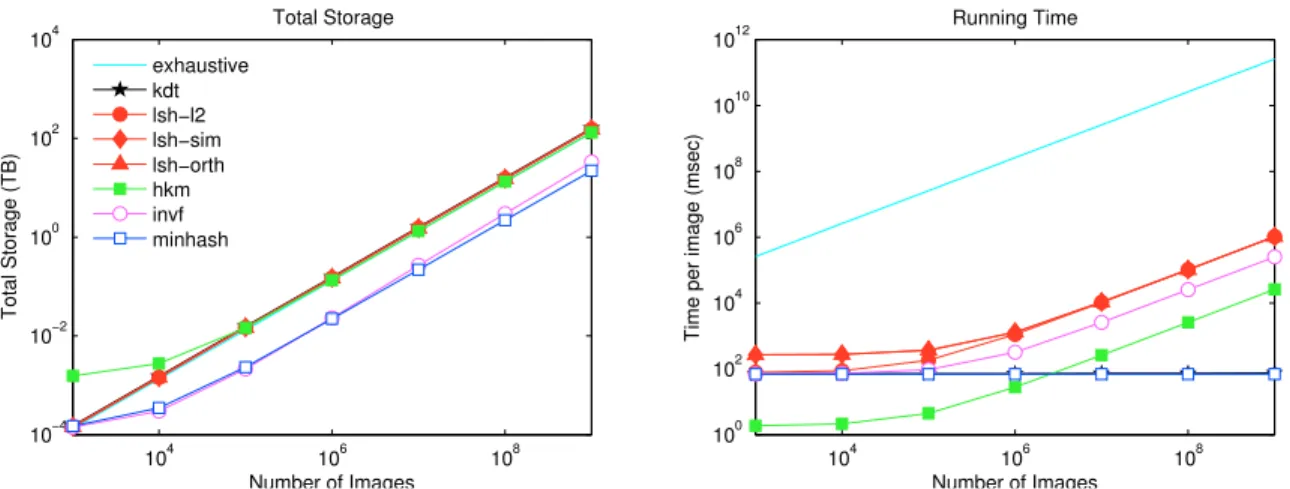
Theoretical Estimates
Theoretical Comparison
- Memory and Run Time
- Parallelization
The root machine stores the top of the tree, while the leaf machines store the leaves of the tree. We call this approach Distributed Kd-Trees (DKdt), since different parts of the same Kd-Tree are distributed on different machines.
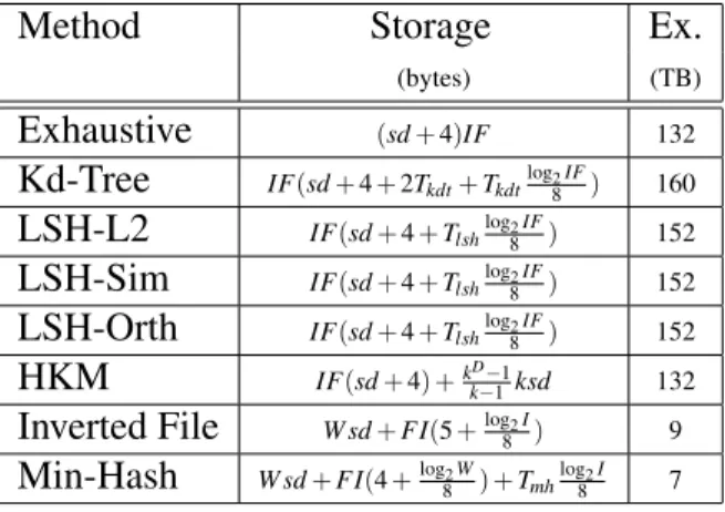
Theoretical Derivations
- Exhaustive Search
- Kd-Trees
- Locality Sensitive Hashing (LSH)
- Hierarchical K-Means (HKM)
- Inverted File (IF)
- Min-Hash (MH)
Speedup: Having more machines here equates to linearly speeding up the search process (in the number of images). Speedup: Having more machines here equates to logarithmic speedup of the search process. The central machine(s) will get query functions, traverse the top of the tree, and then send functions to the appropriate node machines.
Summary
Introduction
Datasets
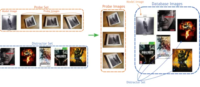
- Probe Sets
- Distractor Datasets
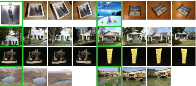
The first image in each group is the model image and the rest are the probe images. Each row shows the number of model images, number of probe images, and total number of images. A set of ~400K images of “objects” collected from www.image-net.org, specifically images under synsets: instrument, furniture and tools.
Experimental Details
- Setup
- Parameter Tuning
The ranking before the geometric check is based on the number of closest objects in the image, while the ranking after the geometric check is based on the number of inliers of the affine transformation. In our setup we have only ONE correct ground truth image to retrieve and multiple probe images, while in the other setting there are a number of images that are considered correct. This database would have one canonical image for each book and the goal is to correctly identify the book in the probe image.
Experimental Results and Discussion
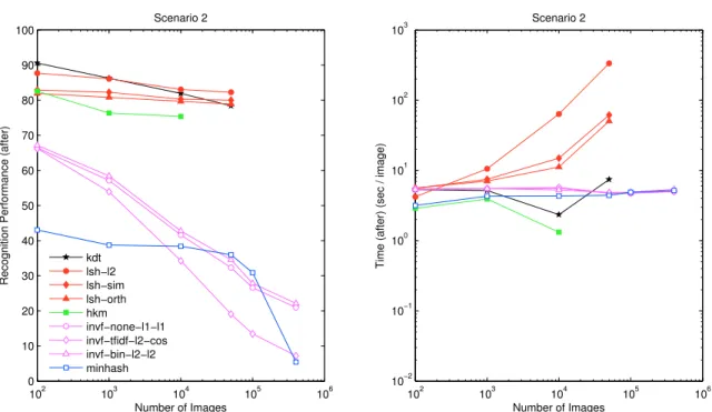
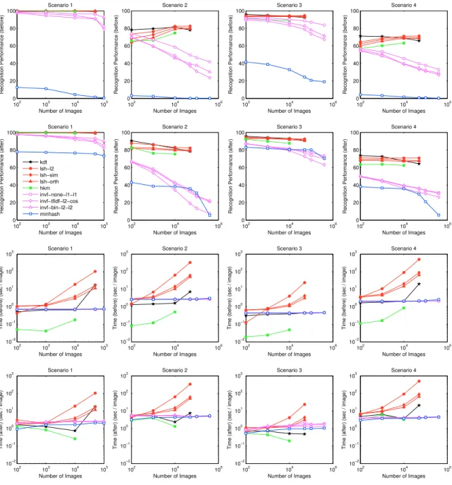
For more detailed results, please refer to Figure 4.8. the main memory, see the big jump in Figure 4.7 for 50 K images) that provides logarithmic increase in seek time. Spherical LSH methods offer a comparable recognition rate to LSH-L2 methods, but they offer better search time. Furthermore, with clever and more complicated parallelization schemes, such as the one described in Section 3.3.2 and Figure 3.3, we can have significant speedups when running on multiple machines.
Parameter Tuning Details
- Kd-Tree
- Locality Sensitive Hashing
- LSH-L2
- Hierarchical K-Means
- Inverted File
- Min-Hash
We then decided to use four tables with five and seven hash functions, the results of which are shown in Figure 4.11(b). We then decided to use four tables with five and seven hash functions, the results of which are shown in Figure 4.12(b). Based on the results, we chose AKM dictionaries with 1 million visual words and the three combinations {tf-idf,l2,cos}, {bin,l2,l2} and {none,l1,l1} for the full alignment in Figure 4.15.
Summary
Introduction
Finally, we compare our method with the state-of-the-art Hamming Embedding BoW method [20] and report better performance with equivalent or less memory.
Compact Binary Signatures
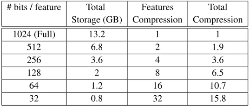
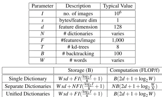
The second column shows the memory used when compressing SIFT features with binary signatures of different lengths using FM Kd-trees with typical parameter values in Table 5.1. Build a set of Kd-trees{Tt(fi j)}using the full set of features{fi j}, then store only the set of binary signatures{bi j}. Instead of using full SIFT features, we can instead calculate binary signatures or PCA and use them instead.
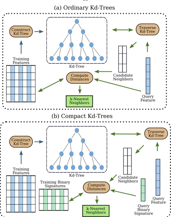
Compact Kd-Trees (CompactKdt)
Given a query attribute, the tree is traversed for candidate nearest neighbors using the full query attribute description. We build the Kd-Trees using the complete training features, then these features can be discarded and we store only their binary signatures. At query time, we traverse the Kd trees using the complete query features to get the list of candidate decision features, but only verify the correct nearest neighbor using the binary signatures (see Algorithm 5.1 and Figure 5.1).
Experimental Results
- Setup
- Binary Signature Comparison
- Compact Kd-Tree
- Comparison with Bag of Words
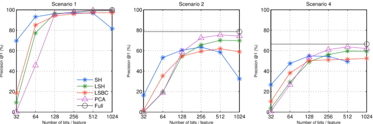
This significantly improves performance while using exactly the same storage and computation cost as using binary signatures with conventional Kd trees (see Table 5.2 and Section 5.2). Black circles show performance using all features (128 bytes), while blue stars show SH with regular Kd trees providing the best performance from Figure 5.2. CompactKdt achieves significant performance improvements over using binary signatures with conventional Kd trees while using the same storage.
Summary
Introduction
Multiple Dictionaries for Bag of Words (MDBoW)
The second term increases linearly with the number of entries in the inverted file, which is controlled by the number of images and the number of distinct dictionaries N. This is because the dominating factor is the backtracking in the set of trees Kd (the first two terms in formula in the third column in Table 6.1), while the depth traversal of the tree (the last term) increases only logarithmically with the number of words. The storage of SDs increases linearly with the number of dictionaries as the entries in the inverted file multiply.
Experimental Details
- Setup
- Bag of Words Details
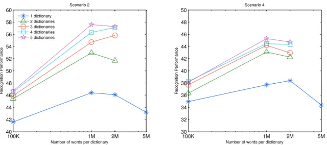
We find that the cost (in memory and computing power) of SDs increases linearly with the number of dictionaries, independently of the number of words. Also, the cost of UDs is virtually independent of the number of words, comparable to a single dictionary. Note that simply increasing the number of words in a single dictionary (blue) is still worse than both SDs and UDs.
Experimental Results
- Multiple Dictionaries for BoW (MDBoW)
- Model Features
- Putting It Together
We plot the baseline IF with/without model functions and the HE IF with/without model functions. We note that combining model features with MDBoW using either Baseline IF (green) or HE IF (cyan) significantly improves performance over not using them (blue and red). Furthermore, combining the model features with MDBoW using HE (black) gives about 65-75% performance increase over Baseline IF with 1 dictionary (blue) and about 25-38% performance increase over HE with 1 dictionary ( cyan).
Summary
For Hamming Embedding IF, using MDBoW with HE without model features (magenta) gives a performance increase of ~32% compared to the state-of-the-art HE with 1 dictionary (cyan).
Introduction
MapReduce Paradigm
The Reduce function summarizes these values and outputs for each word the number of times it appeared in the input document. For each word in the line, it outputs an intermediate pair with the word as the key and a value of "1". MapReduce takes care to group all intermediate pairs with the same key (word) and presents them to the Reduce function, which simply sums the values for each key (word) and outputs a pair with the word as the key and the number of times that word appeared as the value .
Distributed Kd-Tree (DKdt)
At query time, the root machine routes functions to a subset of the leaf machines, leading to higher throughput. This is justified by the fact that most calculations are carried out in the blade machines [3]. The notable difference from IKdt is Feature MapReduce, which builds the top of the Kd tree.
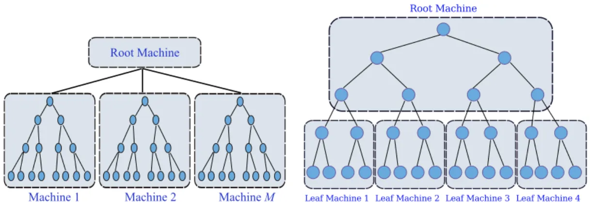
Experimental Setup
On M machines, the upper part should have Kdt⌈log2M⌉levels, so it has at least Mleaves. Index MapReduce builds the lower parts of the tree, where the index map directs the database functions to the Kdt that will own it, which is the first leaf of the upper part that the function reaches with a depth-first search. Specifically, precision@k= ∑#queriesq{rq≤k}, where rq is the resulting ground truth image rank for the query imagebeqin{x}=1 if{x}istrue.
Experimental Results
- System Parameters Effect
- Results and Discussion
We observe that the recognition performance of DKdt remains almost constant with different number of machines as the throughput increases. For DKdt, this determines the number of levels in the upper part of the tree, which is trained in Feature MapReduce, Section 7.3. We note that throughput multiplies by increasing the number of root machines, which provide multiple entry points to the recognition system.
Summary
The different curves show different compression values for compact distributed Kd trees: using 64 bits, 96 bits and 128 bits per feature.
Conclusions
Use more than one Kd-Tree in the Distributed Kd-Trees system, which can increase the accuracy at the cost of using more memory. We provide a comprehensive comparison of the two leading image indexing approaches: Full representation and Bag of words. The system outperforms the state-of-the-art in both recognition performance and throughput, and can process a query image in a fraction of a second.