Impact-induced damage and fracturing would result in an extensive reduction in compressional wave velocity in the recovered target below the impact crater. Impact damage is measured by mapping the reduction in compression wave velocity in the recovered target.
Background
However, impact-induced damage beneath impact craters as a potential constraint has not yet been systematically investigated. In this work, the study of impact damage under craters is carried out at the cm scale in the laboratory.
Organization of this dissertation
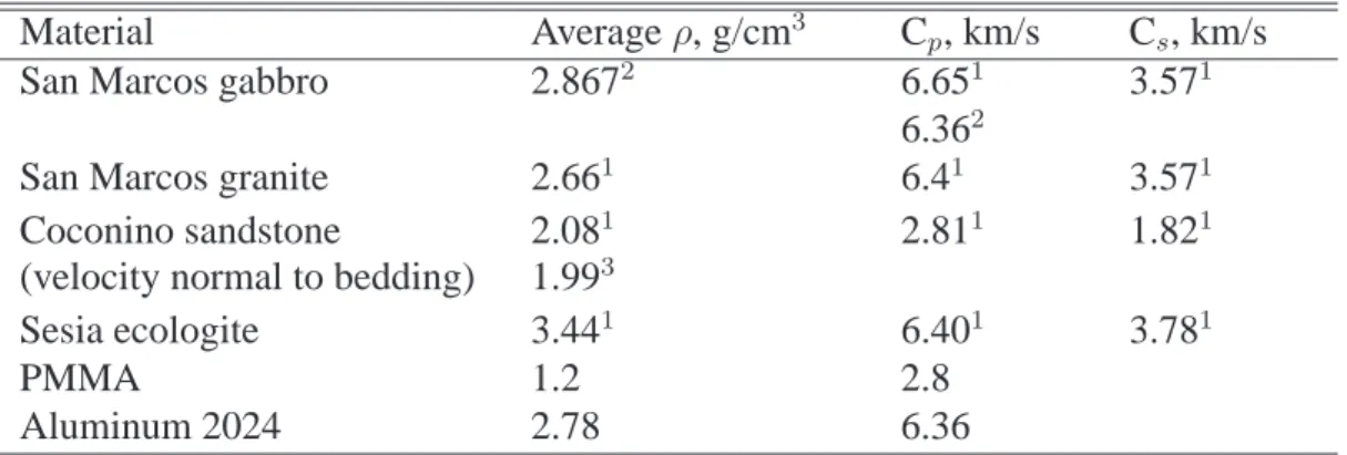
For this reason, ultrasonic method 3 has been chosen to determine the tensile strength in this work. In this study we selected two igneous rocks (San Marcos gabbro and granite), one sedimentary rock (Coconino sandstone) and one metamorphic rock (Sesia eclogite) for dynamic tensile strength determination using method 3 above.
Significance and lithologies of rocks
Mineralogical composition obtained by scanning electron microscopy (SEM) of the thin section for San Marcos granite is shown in Table 2.1. The dynamic tensile strength of Coconino Sandstone from Meteor Crater, Arizona is of interest, as Coconino Sandstone is one of the main sedimentary rocks of the crater [Shoemaker, 1963].

Experimental techniques
When the peak tensile stress exceeds the dynamic tensile strength of the rock, cracks begin to appear in the specimen. The achieved parallelism of the sample surfaces was ±0.003 mm for the San Marcos gabbro and the Sesia eclogite.
Results and discussion
Reduction of velocity by cracks
Both radial and face-parallel cracks are expected to contribute to the wave speed reduction. Although we can determine the elastic wave velocity from a given crack distribution, the reverse is not true.
It is impossible to determine the exact distribution of cracks in rocks by elastic wave velocity measurements alone, since the distribution of cracks is not a unique function of velocity [Nur, 1971].
Strain-rate effect
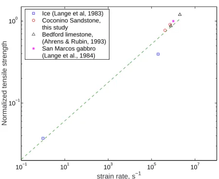
Also included is σc, the tensile strength at a strain rate of 106s−1, extrapolated from available data or measured directly. The dynamic tensile strengths of the Coconino sandstone, normalized by σc, versus strain rate are shown in Figure 2.9.

Conclusion
San Marcos granite, ~20 MPa for Coconino sandstone at 1.4 µs duration, ~17 MPa at 2.4 µs duration, and 240 MPa for Sesia eclogite. Complete fracture occurs above 250 MPa for gabbro and granite, 40 MPa for sandstone and ~480 MPa for eclogite.
Introduction
Experimental procedure
Cratering
Tomography technique
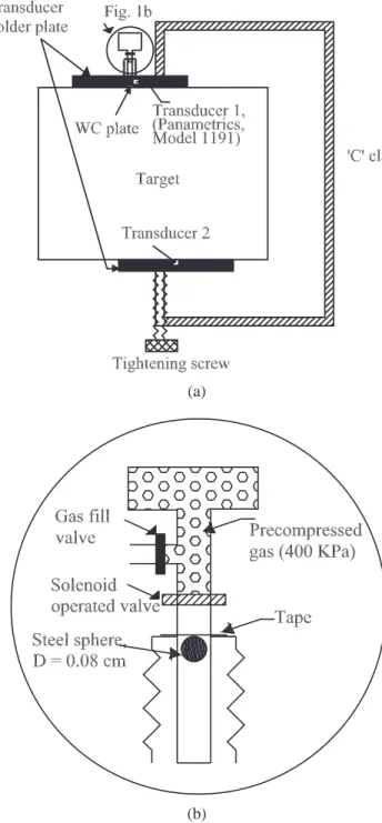
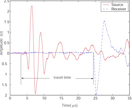
A typical record is shown in Figure 3.2 and the travel time is determined by the time delay between the initial jumps of the two signals. The source and the second transducer are first placed on the two parallel surfaces (left and right, top and bottom) of the target.
Results and discussion
Tomography inversion
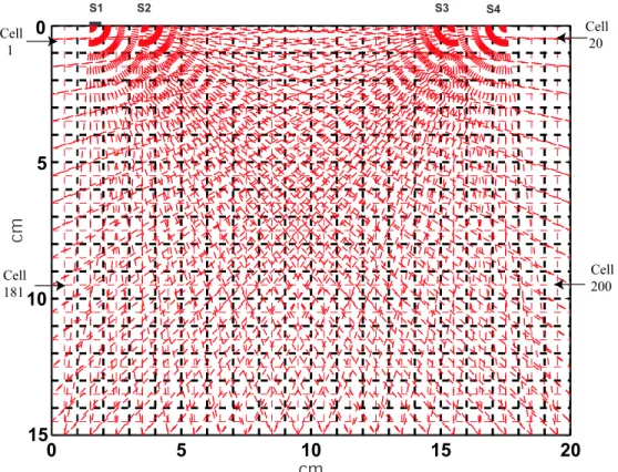
Therefore, eight sources, instead of four, on the upper surface of the rock block, are placed to obtain a complete coverage of the area of interest. Knowing the positions of the source and receiver of each ray and assuming that the ray travels in a straight line from the source to the receiver, Gij can be easily calculated using basic geometry. Therefore, the inversion for the central plane compressional wave velocity is a mixed definite problem.
Test problems
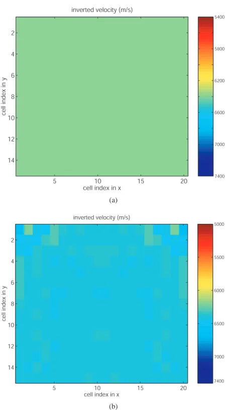
Next, we will discuss how to determine the actual curve beam path in a structure with velocity contrast. To find the actual curvilinear path from one source (S) to one receiver (R), the travel time from S to all the grid points is calculated using the 3-D finite differential package [Hole, 1992] and the velocity model obtained from straight beam assumption as the reference model. Velocity of the 20x15 cm structure is 6.4 km/s and the low velocity zone in the middle is 5.0 km/s; (b) Inverse velocity structure using the tomography method with curvilinear assumption.
Experimental results
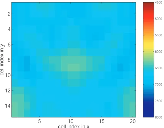
The curved beam from the source to the receiver is slightly deflected from the straight beam path (Figure 3.10c). The diagonal values of the model resolution matrix for each iteration are shown in Figure 3.15. Values of model resolution matrix for cells near the edge are very low, only around 0.1 for these cells (Figure 3.15).
Concluding remarks
Numerous theoretical models have been developed to relate the observed elastic velocity behavior to crack density of the cracked body. Experimental results will then be presented, followed by analysis and discussion of the experimental data. The measured stress wave velocities will be used to calculate the damage parameter and crack density of the fractured rocks.
Experimental technique
The calculated speed has a 2% error, estimated based on the accuracy of travel time and length measurements. The thickness of the intermediate plates is chosen in such a way as to prevent overlapping of waves reflected from different surfaces. With a thin reflector, the first multiple from surface A is observed before the reflected wave from surface B (Figure 4.3b).
![Figure 4.2: Sketch of attenuation measurement system (modified from Winkler and Plona [1982]).](https://thumb-ap.123doks.com/thumbv2/123dok/10413411.0/84.918.243.730.501.864/figure-sketch-attenuation-measurement-modified-winkler-plona-1982.webp)
Experimental results
Compressional wave velocity measurements
The ultrasonic P-wave velocity rise to its unshocked value atr/r0 is equal to 20, or the radial distance ~6 cm. This is in good agreement with the observation of the limit of radial cracking that can be seen in the cross-section after cutting the target (Figure 3.17).
Attenuation measurements
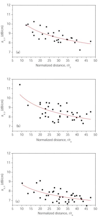
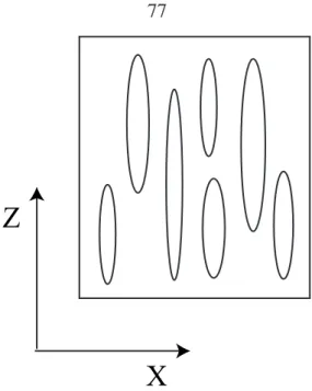
It is evident from Equations 4.6 and Figure 4.8 that at the same distance from the impact point, the attenuation parameters in the z direction are smaller than those in the x and y directions. Therefore, the amplitude of the pressure wave in the z direction weakens less than the amplitude in the directions normal to the orientation of the tensile cracks. This is because tensile cracks mostly extend in the z direction and the effect of cracks on the amplitude of the ultrasonic wave is greater in the directions normal to the crack orientation, which are the x and y directions, than in the direction along the crack orientation.
Analysis and discussion
The intercepts of these equations represent the intrinsic values of the damping coefficients of the samples when no shock-induced damage has occurred (D equals zero). However, the slope of the equation for z direction is only about half of the values of x and y directions. More work should be done in the future to obtain additional information about the microstructure of the investigated media.
Concluding remarks
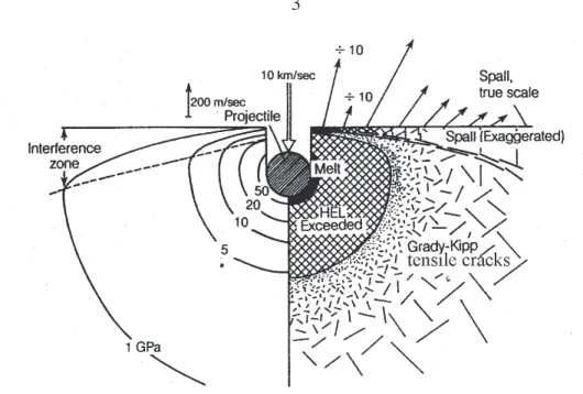
The formation of an impact crater is a combined effect of impact size and material, impact velocity, target material properties, and other variables such as local gravity. Preliminary work has been done to study damage and cracking under craters in the laboratory recently [e.g. It has been suggested that the rupture information for the impact crater is a very useful constraint on the impact history [Ai and Ahrens, 2004].
Dimensional analysis
The left side of the equation can be replaced by the crater volume, crater depth and radius, ejection, etc. When the projectile is a kilometer size, the effect of gravity is large compared to the strength of the target, the expletive is ignored ("gravity regime"). Again, the left side of Equation 5.5 can be replaced with other measurements of the impact crater, such as crater depth, ejection velocity, etc.
Experimental data and discussion
For the rest of the analysis, it is convenient to use this value instead of the true projectile radius a. Based on the dimensional analysis in the previous section, the damage depth of the craters listed in Table 5.1 is normalized by the apparent projectile radius, apa, via the projectile-to-target density ratio plotted against the strength parameter, π3, as shown in Figure 5.3. The slope of the fitted line is -1.27, which corresponds to a µas value of 0.8 according to equation 5.5.

Summary
Information of shock-induced damage and cracking beneath impact craters is an important constraint on impact history. However, no attention has yet been paid to the shock-induced damage under oblique impact craters. This study presents results from laboratory oblique impacts designed to measure the shock-induced damage under impact craters.
Experiments
Results and discussion
Experimental results
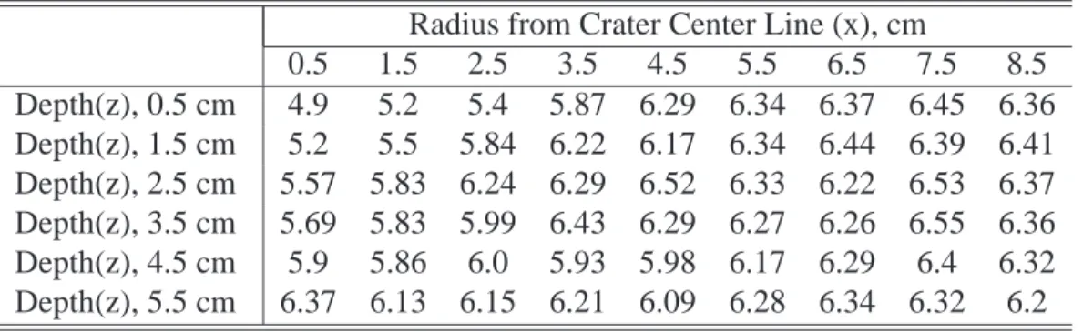
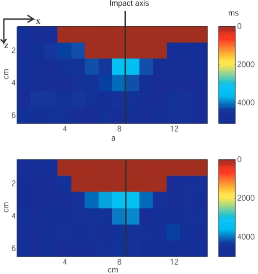
The asymmetry is observed, although not very obvious, for the inverted pressure wave structure of Plane A, the plane containing the projectile trajectory (Figure 6.3a). Similarly, the asymmetry of the low-velocity zone is observed in plane A, the plane containing the projectile trajectory, and higher velocity reduction is observed along the lower boundary (Figure 6.4a). A-plane and B-plane compression velocity measurements for reclaimed Bedford limestones using the dicing method are listed in Tables 6.1 and 6.2 and shown in Figures 6.5 and 6.6.

Discussion
They also found that an asymmetric peak stress pattern occurs when the impact angle is as high as 45o; the peak downward stresses are nearly twice as large as the upward stress at the same distance, even in the far field from the point of impact (Figure 7 in Dahl and Schultz [2001]). It should be noted that the measurements in this study are performed in the strength regime when the influence of gravity is neglected. For kilometer-sized impact craters in the field, the result in this paper may not be directly applicable, since then gravity would play an important role.
Conclusion
Although experimental parameters such as impact velocity, projectile and target materials, and impactor orientation can be varied over a wide range in the laboratory, the full range of parameters of interest cannot be measured, especially for the large, gravity-controlled craters. in the solar system, are varied. achieved experimentally. In the next session we will discuss AUTODYN, the package used for simulation in this work [AUT, 2003]. We explain in detail how to determine appropriate JH-2 model parameters for granite based on experimental data in the literature.
Related work
An overview of AUTODYN
Description of brittle material model
- JH-2 model
- Tensile crack softening model
The crack softening model simulates a gradual decrease in the capacity of brittle materials at a late stage when the magnitude of the principal tensile stress is of the same order as the shear stress. In AUTODYN, the crack softening model is implemented as follows: at failure initiation, the current maximum principal tensile stress in the cell is stored. A linear softening slope is then used to define the maximum possible principal tensile stress in the material as a function of the crack strain.
![Figure 7.1: Description of JH2 model for brittle materials (from Johnson and Holmquist [1999], Figure 1).](https://thumb-ap.123doks.com/thumbv2/123dok/10413411.0/144.918.192.791.212.899/figure-description-model-brittle-materials-johnson-holmquist-figure.webp)
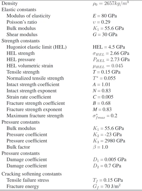
Determination of model constants for granite
- Pressure
- Strength
- Damage
- Tensile cracking softening
This softening slope is a function of the local cell size and the fracture energy (the energy required to create a unit fracture surface) of the material, Gf. The difference between the axial stress and the pressure is an indication of the strength of the material. We assume the magnitude of the tensile stress is equal to that of the original compressive stress.
Examples
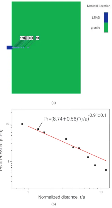
- Lead bullet impacting granite
- Copper ball impacting granite
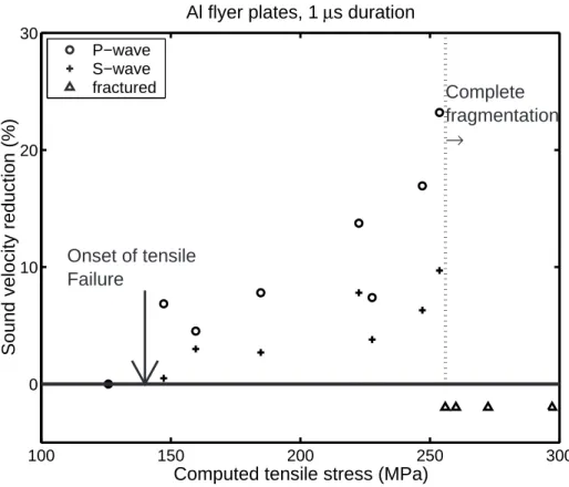
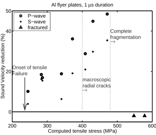
- Plate impact of Al flyer plate into granite
- Oblique impact
- Effect of gravity on damage and cracks
For convenience, the cross section showing different types of cracks and depth of damage is shown again (Figure 7.7a). For the weak-moderate impact with impact velocity U = 15.6 m/s, only initial and few well-developed short cracks are observed (Figure 7.9b). The pattern of damage and tensile cracks in Figure 7.11 is in good agreement with that measured directly (Figure 7.10).
Conclusion
It is also true that many questions are left unexplored in simulation. 1962), Interpretation of lunar craters, in Physics and Astronomy of the Moon, edited by Z. 1989), Strength of rock, in Physical properties of rocks and minerals, vol. Christensen (2001), Ultrasonic p- and s-wave attenuation in oceanic basalt, Geophys. 1987), Elastic properties of rocks and minerals, in Methods of experimental physics, edited by C.
One-dimensional impact setup showing recovery tank, sample, and alignment. 10
Velocity measurements for San Marcos gabbro experiments
Velocity measurements for San Marcos granite experiments
Velocity measurements for Sesia eclogite experiments
Velocity measurements for Coconino sandstone experiments of duration time
Velocity measurements for Bedford limestone. (a) 0.5 µs and (b) 1.3 µs
Normalized tensile strengths as a function of strain rate for ice and rocks
Typical ultrasonic source and receiver signal

![Figure 2.7: Velocity measurements for Bedford limestone. (a) 0.5 µs and (b) 1.3 µs. (From Ahrens and Rubin [1993], Fig](https://thumb-ap.123doks.com/thumbv2/123dok/10413411.0/44.918.181.782.152.941/figure-velocity-measurements-bedford-limestone-ahrens-rubin-1993.webp)
![Antiproliferative Activity of Ethanolic Extract of Ciplukan Herbs (Physalis angulata L.) on 7,12-Dimethylbenz[A]Nthracene-Induced Rat Mammary Carcinogenesis](data:image/gif;base64,R0lGODlhAQABAIAAAP///wAAACH5BAEAAAAALAAAAAABAAEAAAICRAEAOw==)