Inamori School of Engineering Faculty Scholarship
2021-08
Short-term nodal load forecasting based on machine learning techniques
Lu, Dan
Lu, D, Zhao, D, Li, Z. Short-term nodal load forecasting based on machine learning techniques.
Int Trans Electr Energ Syst. 2021; 31( 9):e13016. https://doi.org/10.1002/2050-7038.13016 Wiley
https://doi.org/10.1002/2050-7038.13016
https://authorservices.wiley.com/author-resources/Journal-Authors/licensing/self-archiving.html#3
This is the peer reviewed version of the following article: Lu, D, Zhao, D, Li, Z. Short-term nodal load forecasting based on machine learning techniques. Int Trans Electr Energ Syst. 2021; 31(
9):e13016, which has been published in final form at https://doi.org/10.1002/2050-7038.13016.
This article may be used for non-commercial purposes in accordance with Wiley Terms and Conditions for Use of Self-Archived Versions.
Downloaded from AURA: Alfred University Research & Archives
Short-term Nodal Load Forecasting Based on Machine Learning Techniques
Dan Lu1, Dongbo Zhao2, Zuyi Li3
1Alfred University, 1 Saxon Drive, Alfred, NY, 14802, USA
2Argonne National Laboratory, 9700 S Cass Ave, Lemont, IL 60439, USA
3Illinois Institute of Technology, 35 W 33rd St, Chicago, IL 60616, USA Correspondence
Dongbo Zhao, Argonne National Laboratory, 9700 S Cass Ave, Lemont, IL 60439, USA Email: [email protected]
Summary: This paper introduces an advanced Short-term Nodal Load Forecasting (STNLF) method that forecasts nodal load profiles for the next day in power systems, based on the combined use of three machine learning techniques. Least Absolute Shrinkage and Selection Operator (LASSO) is employed to reduce the number of features for a single nodal load forecasting. Principal Component Analysis (PCA) is used to capture the features of historical loads in low-dimensional space compared to the original high-dimensional load space where features are barely possible to depict.
Bayesian Ridge Regression (BRR) is utilized to decide the parameters of the prediction model from a statistics perspective. Tests based on modified PJM load data demonstrate the effectiveness of the proposed STNLF method compared to the state-of-the-art General Regression Neural Network (GRNN) method. Moreover, the reliability of the day-ahead Unit Commitment (UC) solution is shown to have been improved, based on the forecasted load data using the proposed STNLF method.
KEYWORDS: Least Absolute Shrinkage and Selection Operator (LASSO), Principal Component Analysis (PCA), Bayesian Ridge Regression (BRR), General Regression Neural Network (GRNN), Short-term Nodal Load Forecasting (STNLF), Unit Commitment (UC).
1. INTRODUCTION
POWER systems, as the largest man-made systems, deliver electricity to more than six billion people around the world. However, unlike other commodities, electricity cannot be stored massively and economically with existing technologies, creating the requirement of balancing its generation and consumption at every moment [1] which puts much pressure on the short-term operation of power systems.
This paper is focused on Short-term Nodal Load Forecasting (STNLF) for the next 24 hours, which is critical to the short-term operation of power systems. Because of dramatic climate changes, extreme weather conditions happen more often, leading to new historical high-temperature records every year and extremely cold weather events as well. Hot weather leads to high air-conditioner usage and is the main cause of the peak loads in power systems. Peak load forecasting has been studied often [2-5] and extensively using conventional approaches [2, 4] and innovative methods for a long time [3, 5].
Nodal load forecasting and regional load forecasting have been analyzed in [6-9] to estimate the load behavior based on historical data including load and weather. Nodal load is the key for Independent System Operators (ISOs) in planning and regulating day-ahead system operation. Nodal load forecasting of distribution networks was studied considering the changeable patterns and lack of precise data of multinodal loads [6]. The pattern recognitions showed in [6] reveal one important property of load, that load has a pattern as people act similarly every day and business and industry areas show similar trends in electricity usage; also, the lack-of-precise-data problem is important because missing and false data are common in digital systems, caused by communication and transmission issues. In this paper, patterns are
recognized, and reduced data are employed to express the patterns in a better way;
data cleaning, filling, and correction are utilized as well to fix the data-related issues.
In [7], multinodal load forecasting is solved by the General Regression Neural Network (GRNN) method in two ways: 1) forecast individual nodal loads separately;
2) forecast the total load and use the load participation factors to distribute the load for each node. Both of these two options actually forecast the load only once, which lacks consideration of the relationship between different nodes along with the weather in close areas. In this paper, the authors will consider the relationships among all possible factors which do affect load either by season in the long term or by day in the short term.
In [8], the temperature is included in the load forecasting methods using the Least Absolute Shrinkage and Selection Operator (LASSO) technique, which is proposed to utilize the loads of those physically connected countries in the forecasting model. The idea is employed in this paper as the first step in screening data from different
categories—not only temperature data, but wind speed, dew points, and other possibly related properties are included—and further in dimension reduction to improve the selected data which further reduces the data fed into the final forecasting model. In [9, 10], the importance of feature selection is highlighted because it can reduce the computational burden and contribute to the prediction. The selection has relevancy and redundancy issues which are solved by proposed strategies. We use LASSO to figure out the two problems together by adjusting the parameters that balance the accuracy and computational time.
Several traditional techniques were applied on the short-term load forecasting (STLF), which are compared in [1,11, 12], such as Multiple Linear Regression,
Stochastic Time Series, General Exponential Smoothing, State Space with Kalman Filter Method, and the Knowledge-Based Approach. Modification of traditional methods such as Auto-Regressive Moving Average (ARMA) [13] and an adaption of the multiplicative Auto-Regressive Integrated Moving Average (ARIMA) [14] are used. Most of these approaches are linear, so while simple and efficient, a higher accuracy is hard to reach because they have difficulty capturing the nonlinear part of the load variation.
Recently, machine learning has been used in load forecasting to achieve higher accuracy [15]. The techniques include the optimized combination of Support Vector Machine (SVM) and Wavelet Neural Network (WNN) [16], fuzzy-neural models [11], Artificial neural networks (ANN), Box-Jenkins transfer functions, and Artificial Intelligence (AI) [4]. Other more complex learning algorithms are also introduced in load forecasting, such as Long Short-term Memory (LSTM) Recurrent Neural
Network (RNN)-based frameworks [17], Reinforcement Learning (Q-Learning) [18], and Convolutional Neural Networks (CNN) [19]. Also, an existing method was improved. In [7], load forecasting based on GRNN was reviewed and improved as the C-GRNN, M-GRNN, and MR-GRNN methods. In these improvements, part of the input is not discarded to reduce the computational burden and improve the accuracy for normal days, and all of the inputs are used for holidays. Pointwise prediction is done by all the modified GRNN methods, which does not consider the relationship between nodal nodes and other factors. Overfitting and overparameterization are two major problems in neural network design, and standard benchmarks should be set in this kind of forecasting method. These load forecasting methods are single-scenario forecasting techniques, while the proposed method in this paper is multiple-scenario forecasting. In [7, 20, 21], load forecasting was done by GRNN, and the improved methods proved to provide good results. The GRNN approach is employed as a point of contrast in this paper because of its outstanding performance in capturing both linear and nonlinear properties.
In [22], the next-day load forecasting was done by the multi-equation regression model, and the Bayesian model was used to select the parameters in the model. In [23], the Bayesian approach was also used to select parameters for an autoregressive method for modeling and forecasting a day-ahead electricity load. However, the researchers used the original dimension data to do the modeling, which has a high computation burden and may jeopardize accuracy. Also, only historical load,
temperature, and weekday information were selected as the sources, which is hard to grab other important patterns beside the weekdays or not feature. Finally, they used only single-scenario forecasting, which does not take full advantage of the Bayesian treatment.
As information collection methods improve, huge amounts of data are being collected for use in load forecasting, but it is very hard to find all the relationships among those massive data. In [24], Principal Component Analysis (PCA) was used to conduct dimension reduction to simplify the input of the forecasting process, which is
one of the big issues in practical applications. PCA is also employed in this paper after filtering the features listed before.
The multi-block-based prediction method is applied to load forecasting in both [25]
and [26]. The method of selecting the feature and final target that improve the operation and planning in the power system is similar to the idea proposed in this paper. The problems with these papers are also limited by the use of single-scenario prediction, and the idea of a complex prediction approach will lead the results to an overfitting problem (which is what the authors of this paper are trying to avoid). In [27], the uncertainty of the prediction is the main concern, which resembles the proposed method here. To have a more reliable system, a higher price will be paid, and this is the idea of the trade-off between the reliability and economics of the UC problems. In [28, 29], the uncertainties of the energy sources, energy market price, energy bidding price and demands are considered. When they are trying to become more reliable, the higher payment happens, and this is worthful to prevent the possible outages. With the similar thought, this paper introduces the methods to have multiple predictions for one day and use all these possibilities to find the UC with the least cost. The target is to have a reliable and economical UC.
When conducting the STNLF, if all nodal loads and weather information are considered for one nodal load forecast, 1) the model will be complex, 2) a larger amount of data will be required for training the model, 3) the computational time will be long, and 4) irrelevant nodal load and weather data will jeopardize the accuracy of the result. Thus, we need to identify only a small number of relevant features that can well represent the nodal load. In this way, 1) the model will be simplified, 2) the data requirement will be small, 3) the computation will be easier, and 4) the accuracy will be improved. The authors collect, purify, and simplify data by gathering different kinds of resources and filtering out the highly related features by applying LASSO from the data-only point of view. Then the key information is extracted by PCA. As a result, the computation time is reduced, the irrelevant features and smear of
information are ignored to avoid overfitting, and the accuracy is improved.
The contributions of this paper are:
1) Generate a set of predictions instead of the most accurate one: We use Bayesian Ridge Regression (BRR) to obtain a set of the coefficients in order to get a set of prediction results. This set of predicted values can compensate for the volatilities of the load. In comparison, GRNN (same situation for other methods) can only generate scenarios by moving the predicted load curve up and down.
2) Serves ISOs: We cast load forecasting under the context of serving as the inputs to the next-day generation scheduling in power systems. We consider a better load forecasting to be one that better optimizes UC (ON/OFF plan for generators), whereas other load forecasting methods target only the lower error of a single forecast. A better UC leads to higher system reliability.
The rest of the paper is organized as follows. Section 2 outlines the proposed STNLF method. Section 3 presents the key algorithms in detail. Section 4 presents case
studies and simulation results that demonstrate the effectiveness of the proposed STNLF method. Section 5 concludes this paper. Section 6 is the acknowledgment.
2. OUTLINE OF THE PROPOSED STNLF METHOD
In [30], the nodal loads are obtained by multiplying the total load by bus load distribution factors (LDFs) after loads are sorted by the similarity of substation loads.
The disadvantage of this method of predicting total load and distributing nodal loads is that nodal loads do not always strictly follow LDFs. Single nodal load forecasting has the self-evident issue as it does not consider correlations among nodal loads [31].
Our solution to the above problems is STNLF with the following steps. The key algorithms used in this process will be presented in detail in Section 3.
(1) The historical load and weather information of each nodal load are analyzed and extracted by LASSO. The correlations among nodal loads are identified, and the weak correlations are removed from further consideration.
(2) The correlated data are processed for feature extraction by PCA. The purposes are to reduce dimension, explore features, simplify the prediction model, and reduce computational time.
(3) Nodal loads are predicted by an advanced method called BRR based on the reduced data by PCA. The objective is to obtain the hyperparameters that simulate the stochastic nature of the actual loads.
The essential aspects of this flowchart are listed as follows and shown in Fig. 1.
(1) Gather historical load data and weather data including temperature, wind speed, and dew points. There might be additional weather data that are hard to incorporate into the model as they may have too many missing data elements that are hard to fix.
In this paper, the load data are zonal load data obtained from PJM [32]. Weather data are obtained from National Oceanic and Atmospheric Administration (NOAA) [33]
corresponding to the airports within PJM zones. All the data are normalized into the range between 0 and 1, and the maximum values are retained in order to restore the original data. LASSO is then used to find the dependent features and the 𝑅! score (set as 88% initially and might increase up to 100% as needed to find the optimal solution) describes the performance of LASSO.
(2) Perform PCA on selected features from (1). A number of components are chosen in such a way that 95% of the information can be retained (the percentage might be increased up to 99% to find a feasible UC). The basic rule of choosing the
number of dimensions is to achieve a balance between a good approximation and moderate dimension.
(3) Prepare the sample dataset based on the data dimension determined in (2) and include binaries concerning whether a day is a holiday or not and whether a day is a weekday or on the weekend. Arrange every three days (including the reduced data of load and weather, weekday, holiday) in one line to form one sample. In this paper, we use as many samples (4494 samples) as we can to do the forecasting for the next day.
(4) For each load by applying BRR model, train the reduced components one by one and sample 20 sets around the predicted one through sampling the parameters
around the optimal ones. Reconstruct the related feature for each load using the
Fig. 1 Flowchart of STNLF
transform matrix of PCA and get the hourly load profiles corresponding to each load.
The actual loads can be obtained by multiplying the profiles by the maximum values retained in step (1).
3. KEY ALGORITHMS IN THE PROPOSED STNLF METHOD
3.1 Least Absolute Shrinkage and Selection Operator (LASSO)
LASSO was first introduced by Tibshirani in [34], which aims to simplify the linear model. Mathematically, it is a linear model with the 𝑙1-norm for
regularization. The objective is to minimize the least squares with the regularization part of the 𝑙1-norm, which are least absolute deviations and represented by 𝛼‖𝝎‖"
in the following equation [35]:
min
𝝎
"
!$‖𝑿𝝎 − 𝒚‖!!+ 𝛼‖𝝎‖" (1) where 𝑿 is the array of given features, N is the number of data we can gather for the problem, 𝒚 is the vector of the feature we need to predict, 𝝎 is the vector of the weights, 𝛼 is a constant and ‖𝝎‖" is the 𝑙1-norm of the parameter vector. When 𝛼 is sufficiently large, part of the value of the coefficients 𝛚 will be driven to zero and the corresponding features will play no role in the formulation of the target value.
In most cases, the 𝑙2-norm (the least-squares method) is used as a regularization term because of its stable and analytical solution. However, when the existing data have a lot of features that are irrelevant to the target feature, the 𝑙2-norm will lead to a high computation burden. In the meantime, the 𝑙1-norm can extract the most relevant features to get the best representation of the target.
When choosing 𝛼 of Eq. (1), the 𝑅! score is introduced to measure how well the targeted features are represented by other features. The best score is 1.0, and it can be negative when other features are totally irrelevant to the target [32]. The definition is as follows:
𝑅!(𝑦, 𝑦3) = 1 −∑∑#$%!&'('('!(')!)"
!('+)"
#$%!&' (2)
where 𝑦6 =$"∑$(",-.𝑦,.
In Eq. (2), 𝑦, is the kth target feature value, 𝑦3, is the kth value represented by LASSO, and 𝑦6 is the mean of the target feature value. Through setting a threshold (88%) to the 𝑅! score, we can decide the value of 𝛼. And the threshold will increase when the feasible UC is not met.
In this paper, the load data are taken from PJM historical metered zonal loads of years 2000 to 2014 [32]. Weather information is collected from NOAA [33], including temperature, wind speed, and dew points. These weather data from the airports in the PJM area are gathered as different features. LASSO is used to extract the features related to a specific nodal load. The IEEE 30-bus system with 21 nodal loads is considered as the testing transmission system. So, the data of the 21 nodal loads are represented by 21 zones of PJM data. In addition, the weather data from 23 airports are collected in these zones.
The data of the last year will be saved for testing and will not participate in the training. We concatenate 21 nodal loads and 23*3=69 weather features (temperature, wind speed, and dew points from 23 airports) into 90 columns. 𝛼=1 is the default value. If the score of 𝑅! is less than 88% (the initial score), then 𝛼 = 𝛼/2 is used in the next calculation of LASSO until the limit of 0.88 is met. This limit is set to achieve a tradeoff between getting a better representation and having fewer features.
And the limit will increase when the feasible UC is not met.
For the IEEE 30-bus system, features 0-20 are used to represent the 21 nodal loads.
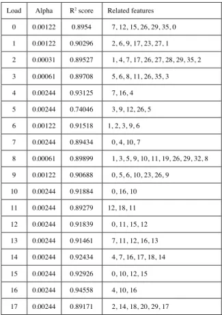
Feature 21-89 are the weather features (temperature, wind speed, and dew points) for 23 airports. Table I shows the related features of each load.
Table I: Related features of each load when the limit is set to 88%
Load Alpha R2 score Related features 0 0.00122 0.8954 7, 12, 15, 26, 29, 35, 0 1 0.00122 0.90296 2, 6, 9, 17, 23, 27, 1 2 0.00031 0.89527 1, 4, 7, 17, 26, 27, 28, 29, 35, 2 3 0.00061 0.89708 5, 6, 8, 11, 26, 35, 3 4 0.00244 0.93125 7, 16, 4
5 0.00244 0.74046 3, 9, 12, 26, 5 6 0.00122 0.91518 1, 2, 3, 9, 6 7 0.00244 0.89434 0, 4, 10, 7
8 0.00061 0.89899 1, 3, 5, 9, 10, 11, 19, 26, 29, 32, 8 9 0.00122 0.90688 0, 5, 6, 10, 23, 26, 9
10 0.00244 0.91884 0, 16, 10 11 0.00244 0.89279 12, 18, 11 12 0.00244 0.91839 0, 11, 15, 12 13 0.00244 0.91461 7, 11, 12, 16, 13 14 0.00244 0.92434 4, 7, 16, 17, 18, 14 15 0.00244 0.92926 0, 10, 12, 15 16 0.00244 0.94558 4, 10, 16 17 0.00244 0.89171 2, 14, 18, 20, 29, 17
18 0.00244 0.88362 11, 14, 17, 18 19 0.00244 0.89957 10, 15, 18, 19 20 0.00122 0.89673 3, 17, 18, 26, 35, 20
It can be observed that some nodal loads are just related to the nodal loads themselves (0-20) and are not related the weather at all. It is probably because the load profiles are coming from PJM zonal data and some zones are composed of several areas. Accordingly, the weather data of just one spot cannot represent the load data of the entire zone. In this case, only those related features are used to do the prediction, such as nodal loads 4, 6, and 7.
Almost all nodal loads can reach the limit of the 𝑅! score, which is set to 0.88.
They can reach an even higher 𝑅! score, but to do so, more features will be selected, which may lead to heavier computation and potentially overfitting. Only nodal load
#5 gets an 𝑅! score of 0.74, which is for the zone DAYTON of PJM. The result indicates that this load is less related to the weather data of Dayton International Airport (DIA), while it is more related to the dew point of Chicago O’Hare International Airport (ORD). In contrast, nodal load #4, the zonal load of
Commonwealth Edison (ComEd), is not related significantly to any weather data of ORD or Rockford International Airport (RFD); both are airports inside the ComEd zone. Therefore, in this case, the nodal load forecasting will just rely on the related loads themselves.
The reconstruction of the data reveals the relationship between different features.
Machine learning techniques are used to dig out the deep relations between different kinds of data, and these relationships are hard to find by human sense which leads to the following problem that Feature 35 is related to nodes 0, 2, 3, and 20 after applying LASSO; this finding reveals that feature 35 has a common feature, that is a good source of reconstructing node 0, 2, 3 and 20.
Preprocessing should be done before any methods are applied to the data. First, missing data should be filled in. We use the average of the two neighbors to fill in any missing data. If multiple blanks exist continuously, an ascending or descending order of data will be filled into the consecutive blanks. Second, outliers are filtered out and replaced using the corresponding logarithmic values instead. Third, data should be converted from nodal loads or weather features of N days and 24 hours to a vector with N*24 elements. In addition, normalization should be done before we use LASSO to find the correlations, because the load levels are different. Without normalization, those nodal loads with high load levels will always have higher impacts than others
with low load levels. For example, the load level of nodal load 3 (100 MW level load) is much higher than the load level of others (5, 10, 15, 20, 30 MW). Experiments show that without normalization, the load of nodal load 3 (100 MW level load) will be a feature that is related to all other loads.
3.2 Principal Component Analysis (PCA)
Many correlated features selected for a specific nodal load through LASSO are highly correlated to themselves. Circulated and duplicated information is an indication of representation by too many data, which may not be helpful for the following prediction [8]. So PCA is chosen to extract the key components and discard the trivial components [36]. After using PCA, a new coordinate is built with the same dimension as the original one, but each dimension is explained by an eigenvalue indicating the variance information of the data on that dimension. After sorting the eigenvalues from large to small, we can decide how many dimensions will be saved by the precision, which can be calculated by ∑0/-"𝜇// ∑$/-"𝜇/ ≥ 𝛿. Here 𝜇/ is the ith eigenvalue, N is the total number of dimensions, 𝛿 is the precision with the range of 0 to 1, and p is the number of dimensions left, which can be found by a given 𝛿.
These p dimensions are called principal components (PCs). More details about PCA can be found in [37].
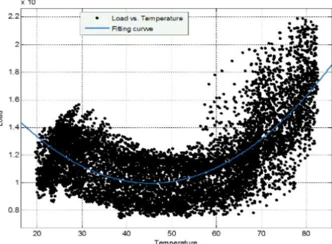
As shown in Fig. 2, load generally changes with temperature. The fitting curve shows that the relationship between load and temperature is approximately quadratic as represented by the blue curve. However, the points around the blue curve are so many that just the quadratic curve is not enough to express the relationship.
Fig. 1 Example of load vs. temperature and their fitting curve ß
of STNLF
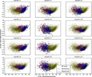
Therefore, PCA is utilized to analyze the load data of a test system with 21 nodal loads for 24 hours, 504 dimensions in total. The top 2 PCs with highest eigenvalues are selected and plotted against each other in the same figure where the x-axis represents the 1st PC and the y-axis represents the 2nd PC. In the monthly plots in Fig. 3, the blue and purple dots show the data for the weekdays and weekends, respectively, in the given month, while the yellow dots represent the data for all load points. The purpose of only selecting two dimensions is for the convenience of visualization and interpretation of the idea. More PCs are used in the actual case study. It can be observed from Fig. 3 that the load data have clear separations for weekdays and weekends in every month. While Fig. 3 only reflects the pattern of the
top two PCs, more useful information can be extracted and will be used to do the actual load forecasting.
3.3 Bayesian Ridge Regression (BRR)
After screening the data to find the related features by LASSO, and then reducing the dimensions by PCA to get the most influential PCs, nodal load forecasting can be done by using Bayesian Ridge Regression (BRR), which is basically a linear
combination of nonlinear kernels with a ridge part to penalize the complexity of the model. Bayesian treatment has been used to find the best parameter when adding the ridge part in [30, 38]. The BRR used in this paper for nodal load forecasting is discussed in detail as follows.
Fig. 3: Load data in 2-dimensional PCA space of STNLF
The goal of regression is to find a proper set of weights 𝒘 to describe the
relationship between one or multiple target values 𝒚 with input data 𝒙 which may contain 1 to D dimensions of variables.
𝒚(𝒙, 𝒘) = 𝜔.+ 𝜔"𝑥"+ 𝜔!𝑥!… + 𝜔1𝑥1 (7) where 𝒚 is the value calculated by the regression method, 𝒘 =
(𝜔", 𝜔!, … 𝜔1)2, 𝒙 = (𝑥", 𝑥!, … 𝑥1). This model is very simple but has many limitations, so the extended form of the linear combination of fixed nonlinear functions of the input variables is introduced:
𝒚3(𝒙, 𝒘) = 𝜔.+ 𝜔"𝜑(𝑥") + 𝜔!𝜑(𝑥!) + ⋯ 𝜔1𝜑(𝑥1) = 𝒘2𝜑(𝒙) (8) where 𝜑(0) is intentionally set to 1 for constructing the matrix form, and 𝜑 is a specific nonlinear function which can be chosen as polynomial, Gaussian, or sigmoidal functions. The Gaussian function is chosen in this paper. In this way, the regression can describe a more sophisticated relationship than the simple linear method.
The next step is to determine 𝒘. The sum-of-squares error (SSE) function is chosen to be the objective:
min "!∑$1-"(𝑡1− 𝒘2𝜑(𝒙𝒏))! (9) which 𝑡1 is the target feature we are expecting, 𝒙𝒏 is the collected features we can use to do the prediction, 𝜑(∙) is the function of 𝒙𝒏 to give more possible combinations between different features, or to use higher orders of the features to dig deeper relationship between features, and 𝒘 is the weight of each 𝜑(∙) function.
To mitigate a potential overfitting problem, a regularization term is added to the objective function, which is normally an 𝑙2-norm represented as . This is called a ridge regression. Accordingly, the new error function is:
min "!∑$1-"(𝑡1− 𝒘2𝜑(𝒙𝒏))!+5!𝒘2𝒘 (10) A proper choice of 𝜆 is not easy, because 1) too large of a 𝜆 will train the model to be too simple to grasp details, 2) too small of a 𝜆 will lead to a complicated model. Bayesian treatment is introduced here to avoid overfitting when minimizing the objective function and to determine the model complexity during the training process in a statistical way [38]. First, assume that 𝑦′(𝒙, 𝒘) has a Gaussian distributed difference 𝛿 with the real value 𝒕 and 𝛿~𝑛𝑜𝑟𝑚𝑎𝑙(0, 𝜎"!). 𝜎 is the standard deviation of a Gaussian distribution. For the later discussion, we define the precision as 𝛽 = 1/𝜎"!.
𝑝(𝒕|𝒙, 𝒘, 𝛽) = 𝑛𝑜𝑟𝑚𝑎𝑙(𝒕|𝑦(𝒙, 𝒘), 𝛽(") (11) w wT
𝛽 is what we want to know in the prediction process. In the analysis, we first consider it as a known parameter to get a set of prior probability distributions of 𝒘 such that 𝒘~𝑛𝑜𝑟𝑚𝑎𝑙(0, 𝜎!!𝑰) which is governed by another precision parameter α = 1/𝜎!!:
𝑝(𝒘) = 𝑛𝑜𝑟𝑚𝑎𝑙(𝒘|0, 𝛼("𝐼) (12) where 𝑰 is the identity matrix. The posterior probability distribution (will use posterior for short in the following paper) of 𝒘 should also be Gaussian with mean 𝒎$ and covariance 𝑺$. The posterior of 𝒘 is proportional to the multiplication of the likelihood function and the prior probability distribution (will use prior for short in the following paper) of 𝒘. Since we select a conjugate Gaussian prior distribution, the posterior of 𝒘 also should be Gaussian. The analytic expression can be derived for conjugate priors, the posterior which is a Gaussian distribution that will be updated with the data coming in. Based on the calculation in [38], we have the
posterior in the following form having mean 𝒎$ and covariance 𝑺$ for the model parameter 𝒘 given the target 𝒕:
𝑝(𝒘|𝒕) = 𝑛𝑜𝑟𝑚𝑎𝑙(𝒘|𝒎$, 𝑺$)
= 𝑛𝑜𝑟𝑚𝑎𝑙(𝒘|𝛽𝑺$𝜱𝐓𝐭, (𝛼𝐈 + 𝛽𝜱𝐓𝜱)(") (13) 𝜱 is the matrix form of 𝜙. If the number of the data is zero, we will keep the distribution of 𝒘 as the prior. And the maximum weight of the posterior will depend on the given number of data while the number is extremely big, and we can have the 𝒘 set as 𝒘𝑴𝑨𝑷= 𝒎𝑵. If we have sequential data, the posterior will change to the prior for the next data coming in.
Transforming (13) to the log of the posterior of 𝒘 turns out to be a summation of the SSE. Selecting the 𝑙2-norm with a coefficient, we have:
𝑙𝑛 𝑝 (𝒘|𝑡) = −;!∑$1-"{𝑡1 − 𝒘2𝜙(𝑥1)}!−<!𝒘2𝒘 + 𝑐𝑜𝑛𝑠𝑡 (14) Then, making the convolution of (11) and (13), we can get the distribution of the next target 𝜏 with new input 𝒙:
𝑝(𝜏|𝒙, 𝒕, 𝛼, 𝛽) = c 𝑝(𝜏|𝒙, 𝒘, 𝛽)𝑝( 𝒘|𝒙, 𝒕, 𝛼, 𝛽)𝑑𝒘
= 𝑛𝑜𝑟𝑚𝑎𝑙(𝜏|𝒎$2𝜙(𝒙), 𝜎$!(𝒙)) (15) where the variance 𝜎$!(𝒙) is given by:
𝜎$!(𝒙) = 𝜎"!+ 𝜙(𝒙)2𝑆$𝜙(𝒙) (16) In Eq. (16), the first term is related to the noise of the data, while the second term describes the uncertainty of 𝒘. We can narrow down the posterior distribution by putting in more data. When the data size is large enough, the uncertainty will go away
and the second term of Eq. (16) will be zero. Under this situation, Eq. (16) is left only with the variance of noise which is controlled by 𝛽. Then several predictions will come from drawing samples from the posterior distribution hyperparameters of 𝒘.
4. CASE STUDIES
This section demonstrates the effectiveness of the proposed STNLF methods using LASSO, PCA, and BRR.
4.1 Test system
The IEEE 30-bus system [39] shown in Fig. 4 is used in this paper as the test system. The details of the IEEE 30-bus system are given in the appendix. It contains 6 generators, 21 loads (as MWs), and 41 transmission lines. 21 zonal loads of the PJM system are selected to represent the 21 nodal loads after adjusting the load level. The nodal loads are taken from PJM historical metered zonal loads of years 2000 to 2014, and the weather data are from NOAA of the same years and related areas. There are 24 hourly load data each day for 21 zones which are adjusted to the load level and assumed to be the nodal loads in this 30-bus system. Weather data from 23 airports are gathered, each with temperatures, wind speeds, and dew points. In total, 90 features are listed as a matrix input for LASSO. More detailed correlated features can be found in Table I.
Fig. 4: IEEE 30-bus system [33]
4.2 STNLF application and results
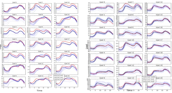
Follow the steps of Section 2, the predictions of each load are plotted in Fig. 5 and Fig. 6, corresponding to two situations (the normal case and the worst case).
The shape of the 21 loads may look similar, which is because of the nature of how people use electricity, but the load levels are different, which can be differentiated by the y-axis of each subplot. The red line is the historical load, the cyan line is the inversed load by the PCA transform matrix, the black line is the expectation of the predicted load, and all the blue dashed lines are possibilities of predicted loads. In the studied case, while the 4494 used samples are large, they are still not enough to assume 𝑁 → ∞, so the model is not only related with the noise but also considered the posterior distribution with random disturbance of 𝒘 by the forecasting precision as well. From Fig. 7, we can see the consideration has its reason because it can cover almost all the load curve and leave only with some minor difference. The predicted load is obtained from the proposed method in which a set of 𝒘 is generated through training the samples for each load. The possible loads (20 scenarios) are obtained from the random sampling of 𝒘 with the mean value of 𝒘 and standard deviation based on the precision of the coefficient 𝒘.
In 95% situations, the proposed method can get very good predictions as the black lines in Fig. 5 show, where most of the real loads and predicted loads are overlapping;
but there are a few cases where the predicted load curve does not follow the actual
Fig. 5: Good performance Fig. 6: The worst performance
historical load curve, as shown in Fig. 6. In these cases, the scenarios will be utilized.
The scenarios are located around the predicted load, and the red curve can be almost covered by the dashed ones with only a few exceptions beyond the range.
365 days of nodal loads are predicted using the proposed method. Even for the worst case shown in Fig. 6, most of the predictions still overlap with the true values.
Some nodal loads, such as loads 7, 10-13, 18, are predicted with lower values at peak.
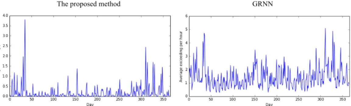
Since those loads all have small load levels, they will not influence the result of the UC too much, as will be discussed later. The left pane of Fig. 7 shows the average overages of real loads from the predicted loads based on the proposed method. It can be observed that the overages are very small in most cases, although some are higher than 4 MW (only 3 cases).
4.3 Ridge Regression (RR)
In [40], the Ridge Regression (RR) was employed to increase the reliability of the ensemble prediction to overcome the small dataset and the results showed the
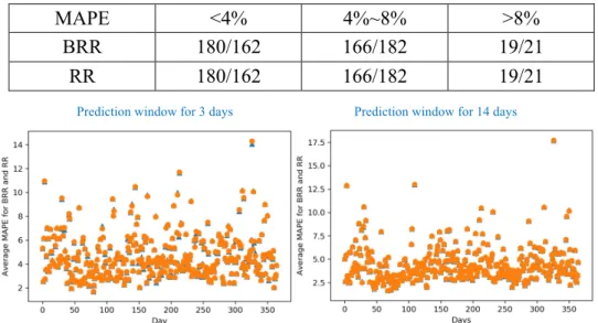
improvement of the prediction accuracy. So, before comparing with the GRNN methods for multiple scenarios, the single predicting results of BRR are compared with the results of RR. The MAPEs of both methods are calculated for a year (365 days with 2 prediction window length). The window length is the days used to do the prediction. From Fig. 8 we can see that only a little difference between BRR and RR from MAPEs’ point of view for two cases. The overall MAPEs average of BRR and RR are 4.437% and 4.433%. Since the RR was used in many other papers and showed the effectiveness, selecting BRR is appropriate. Also, the results reveal that for as long as a year, there are days with quite high MAPEs (lager than 8%), although many days are quite accurate that the MAPEs are low (less than 4%). This triggers the authors to look for the reliable way for the load forecasting.
The proposed method GRNN
Fig. 7: Average overages of real loads from the predicted loads based on the proposed method vs. GRNN
Table II MAPEs of BRR and RR for the case of 14 days/3 days prediction window
MAPE <4% 4%~8% >8%
BRR 180/162 166/182 19/21
RR 180/162 166/182 19/21
Reliability refers to the sensitivity of the predictions to outliers. From the table and the figure in this part we can see that in some days, the predictions cannot be so reliable which lead to high MAPEs with low accuracy. Authors who write about predictions prefer to address how the average accuracy outperformed from other papers. How about those outliers? They are disappeared during the average action.
The comparison just shows how the BRR will be as effective as RR which was proved in other papers, also, it highlights the problem of the outliers, so the multiple scenarios are created in the proposed methods along with the GRNN (showing in the following part) to fill up the missing part about how to deal with the outliers when looking for the UC solutions.
The multiple scenarios are generated in BRR by adjusting the hyperparameters which RR is lack of. This is the reason BRR is used in this paper. Among all techniques to do the prediction, GRNN is another one with a hyperparameter to change which can make multiple predictions. The part enclosed by a dotted green line in Fig. 5 gives an example about changing the hyperparameters in the proposed method is not only an expansion of the upper and lower limit of the best prediction result. Similar situations can be found in Fig. 6 and 10. They show some features found in the model and not shown in the best prediction result. These scenarios cover more possibilities might happen in real life based on the modeling and they benefit in looking for optimal UC solutions.
Prediction window for 3 days Prediction window for 14 days
Fig. 8: Comparison of the average MAPEs for BRR and RR each day for two prediction window length
4.4 General Regression Neural Network (GRNN)
The GRNN method based on the approach of individual forecasts in [41] is used for comparison in this paper. The choice of GRNN is made because of the simple construction of the neural network and its easy implementation with existing modules in Python, as well as its capability of considering outside information such as weather and day type, which is similar to the proposed method. The LDF method is not used for comparison because the nodal loads obtained using that method obviously do not match the real nodal loads.
NeuPy [42], which stands for Neural Networks in Python, is used here for comparison, as it includes the GRNN module. In GRNN, only one parameter, σ, should be adjusted, which is called the spread and is decided by the cross-validation process. The Root Mean Squared Logarithmic Error (RMSLE) is the criterion to decide the best value of σ from a possible list. More details about the construction of GRNN can be found in [41].
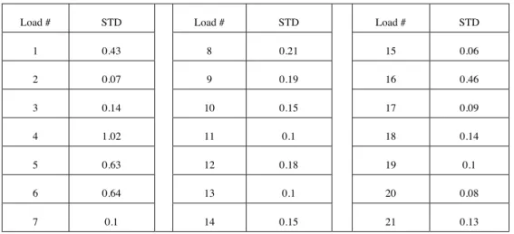
The forecasting can be done after the σ value is decided. To make the comparison fairer, 20 scenarios are also generated by making random changes around the best σ.
5 times the σ value is set as the standard deviation (STD) for getting a bigger prediction area, and the STDs are listed in Table III. Two observations can be made based on the prediction results.
(1) Most results of the GRNN method, the prediction of the same 365 days as the proposed methods did, are good and close to the real values. Some predictions are even better than the predictions made by the proposed method.
(2) The prediction with the best σ always has the best performance compared to all scenarios. In these cases, scenarios are redundant.
Table III: The STD to adjust σ value in GRNN method
Load # STD Load # STD Load # STD
1 0.43 8 0.21 15 0.06
2 0.07 9 0.19 16 0.46
3 0.14 10 0.15 17 0.09
4 1.02 11 0.1 18 0.14
5 0.63 12 0.18 19 0.1
6 0.64 13 0.1 20 0.08
7 0.1 14 0.15 21 0.13
4.5 Comparison with proposed method in uncommon cases
The accuracy of the prediction is not the final aim of this paper. The reliability of the prediction is. Common cases are easy to predict, but those uncommon cases are not. The comparison in this section is focused on those days that have different patterns, and thus are hard to predict, such as the high temperature that happened in California which triggered power outages across the whole of California; this is an extreme example of the uncommon cases.
The one-day prediction using GRNN is shown in Fig. 9. The performance of the prediction is not as good as the proposed method, which can be found in Fig. 10, especially for the peak load prediction. And the economic losses are happening more often in the extreme cases. Although more scenarios are added and the bigger σ value is used for GRNN, they cannot make up the prediction error. The prediction result of the same day based on the proposed method is shown in Fig. 10, which shows more resilience to bad predictions when scenarios are added.
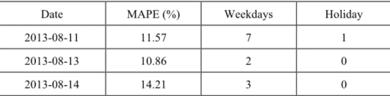
The uncommon cases for the Mean Absolute Percentage Error (MAPE)>10%
(around the days in middle to late August) are filtered out and listed in the following Table IV.
Table IV:The uncommon cases for MAPE>10%
Date MAPE (%) Weekdays Holiday
2013-08-11 11.57 7 1
2013-08-13 10.86 2 0
2013-08-14 14.21 3 0
Fig. 9: Prediction of GRNN Fig. 10: Prediction of the proposed method
2013-08-18 10.31 7 1
2013-08-20 10.1 2 0
2013-08-23 11.22 5 0
2013-08-24 10.78 6 1
2013-08-25 11.03 7 1
2013-08-28 11.01 3 0
2013-08-29 10.6 4 0
The uncommon case predictions are happening around August in 2013, which has the record high temperature [43] at that month for Chicago, Illinois (central America).
The high temperature disturbed the normal forecasting and has very high MAPEs.
The scenarios for these days are very important because more reserves are needed to stand by for the peak load to release the pressure on ISOs. These MAPEs are much larger than the single-scenario prediction; however, they are helpful in making UC decisions with higher resilience.
To make a more in-depth comparison, 15 times of σ is used in the same day.
However, the problem in Fig. 9 is not solved by making this change. The scenarios of prediction seem to spread downwards instead of around the best prediction. This is caused by the non-positive property of σ. When σ is small and close to 0, the random changes of it will be larger than the true value and no change will be smaller than the best value. This is not as flexible as the proposed method and will result in worse predictions.
The right part of Fig. 7 shows the average overages of real loads from the predicted loads of the GRNN method. Although all the overages are quite small and there are no extreme large spikes, there are 33 days when a feasible UC solution cannot be found to meet the load. In this regard, the proposed method has a better performance on obtaining feasible and reliable solutions, as shown in in the next section. The
comparison can be found in Table V, and the infeasible cases are shown in Table VI.
Table V: Comparison of the feasible UC solution for two methods
Method Feasible UC Infeasible UC
The proposed method 365 0
GRNN 332 33
Table VI: The 33 infeasible cases for GRNN
Date Weekdays Holiday Date Weekdays Holiday
2013-08-21 3 0 2014-01-16 4 0
2013-08-30 5 0 2014-01-17 5 0
2013-09-08 7 1 2014-01-18 6 1
2013-09-11 3 0 2014-01-19 7 1
2013-09-12 4 0 2014-01-22 3 0
2013-09-21 6 1 2014-02-02 7 1
2013-10-04 5 0 2014-02-07 5 0
2013-11-08 5 0 2014-02-15 6 1
2013-11-09 6 1 2014-02-16 7 1
2013-11-13 3 0 2014-03-07 5 0
2013-11-19 2 0 2014-03-14 5 0
2013-11-23 6 1 2014-05-17 6 1
2013-12-06 5 0 2014-06-04 3 0
2013-12-08 7 1 2014-06-17 2 0
2013-12-25 3 1 2014-07-04 5 1
2014-01-01 3 1 2014-07-17 4 0
2014-01-12 7 1
4.6 Performance in obtaining feasible UC solutions
In power systems, the ISOs will determine the system UC solutions based on Security Constraint Unit Commitment (SCUC) in order to guarantee the security and optimization of the system [44]. In dealing with the stochastic issues of the load, the Monte Carlo and Robust Optimization are the two key methods to generate the possible load to fight against the net load uncertainty, then use SCUC to optimize the commitment of the generators and find the best commitment for the generators to meet possible load with least cost. By listing the advantages and disadvantages of the two methods below, the decision has been made: not using them and find a third way to avoid the disadvantages. So, this is why we proposed this method. And since the difference of the generating load method, there are no proper ways to do the
comparison with our proposed approach, in the meantime, GRNN has a hyper-
parameter to control the result, so GRNN is chosen to be the method to compare with the proposed method.
Table VII Comparison of different approach to generate load against uncertainty
Advantages Disadvantages
Monte Carlo Generate load randomly as many as possible, use the large number of scenarios to against uncertainty
No logical relationship among hours and time consuming Robust
Optimization
Generate a large band of load with high level of confidence that load will be barely outside the band
Too large of the band leads to high variations (no logical) and high cost
The proposed method
Generate load based on the relationship among hours and use hyper-parameters to control the selections with fewer choices but high confident level
More complex process than others
The model of a UC problem is as follows [44]:
Minimize ∑$>/-"∑$2=-"[𝐹/(𝑃/=)𝐼/=+ 𝑆𝑈/=+ 𝑆𝐷/=] (17) Subject to
∑$>/-"𝑃/= = 𝐷= ∀𝑡 (18)
𝑃?/1,/𝐼/= ≤ 𝑃/= ≤ 𝑃?AB,/𝐼/= ∀𝑖, ∀𝑡 (19)
[𝑋C1,/(=(")− 𝑇C1,/][𝐼/(=(")− 𝐼/=] ≥ 0 ∀𝑖, ∀𝑡 (20)
[𝑋CDD,/(=(")− 𝑇CDD,/][𝐼/=− 𝐼/(=(")] ≥ 0 ∀𝑖, ∀𝑡 (21)
𝑃/=− 𝑃/(=(") ≤ t1 − 𝐼/=u1 − 𝐼/(=(")vw𝑈𝑅/ + 𝐼/=(1 − 𝐼/(=("))𝑈𝑃/ ∀𝑖, ∀𝑡 (22) 𝑃/(=(")− 𝑃/= ≤ t1 − 𝐼/(=(")(1 − 𝐼/=)w𝐷𝑅/ + 𝐼/(=(")(1 − 𝐼/=)𝐷𝑃/ ∀𝑖, ∀𝑡 (23)
|𝑆𝐹 × (𝐾E × 𝑃=− 𝐾F× 𝑃=| ≤ 𝑃𝐿?AB ∀𝑡 (24)
The objective of a UC problem is to minimize the cost of operating generators in a system. The cost includes the fuel cost and startup/shutdown cost in (17). In (17), the function 𝐹/(𝑃/=) = 𝑎/+ 𝑏/𝑃/=+ 𝑐/𝑃/=! is the production cost for all the generators, which is decided by the coefficient a, b, and c. In the equations, 𝑖 is the index of generator, 𝑁𝐺 is the total number of generators, 𝑡 is the index of hour, 𝑁𝑇 is the total number of hours, 𝑃/= is the power production for generator 𝑖 at time 𝑡, 𝐼/= is the ON/OFF indicator for generator 𝑖 at time 𝑡, 𝑆𝑈/= is the startup cost for
generator 𝑖 at time 𝑡, 𝑆𝐷/= is the shutdown cost for generator 𝑖 at time 𝑡.
Load balance (generation = load for every moment) is showing in (18). Real power capacity limits is giving in (19), which means once the generator is opened, it must running at the minimum level and cannot exceed the maximum level. Other limits include minimum ON (20) and OFF (21), generation unit ramping up (22) and down (23) limits, and transmission flow limits (24).
The model can be built based on the given objective and constraints. The solution can be found by applying computer programming with MIP method. Since the test systems are small (less than 118 bus), solving MIP by Gurobi directly is simple. With larger systems, Benders Decomposition will be employed to improve the computation efficiency with less time. The optimal solution is the least cost UC (indicates the ON/OFF status during the modeling time) that no constraint is violated. The feasible solution allows the generators to meet the load during the modeling time. The UC performance is evaluated by the cost after feasibility checking. Part of the flow chart in Fig. 1 describes how to find the best cost among multiple predictions and it works as follows:
Take one flow of this process as an example: one set of predicted load profiles (e.g., 20 in total) and one real load profile:
(1) By setting the objective to minimize the total cost, with the given constraints, calculate UCs for all the predicted load profiles (e.g., use the 20 load profiles to calculate the UC for each scenario).
(2) Take one UC from (1) to identify how many predicted load profiles can be met by this UC (e.g., 16 predicted load profiles out of 20 can be met by the first UC; 20 out of 20 can be met by the second UC, etc.). Check all 20 UCs from (1).
(3) Calculate the cost of the load with highest demand for UCs from (1).
(4) Locate the UC that satisfies the largest number of load profiles with the least cost to be the reliable UC for the next day.
(5) Check whether the best UC can meet the actual load.
365 days of nodal loads are predicted using the proposed method and the GRNN method. For the former method, the result shows that all of the predicted load profiles can determine a UC to meet the real load profiles which is reliable and has relatively low cost. For the worst cases shown in Fig. 6, a UC determination can still be found to meet the actual load, although most of the predictions were underpredicted compared with the true load values (e.g., loads 7, 10-13, and 18). Those load points with large deviations that have small load level leads to less influence on the result.
In comparison, there are 33 out of 365 days of the load predicted by the GRNN method cannot pass the feasibility test (Table V). The failures are caused by the high variations at most nodal loads. This will lead to the unreliability of the UC solution.
5 CONCLUSIONS AND FUTURE WORK
Power system load modeling and forecasting are becoming increasingly crucial to system operators, given the recent challenges of renewable energy integration and cascading failures such as faults induced by or inducing wildfires. Correlations among factors impacting the loading condition are expected to be accounted for in the load management framework. In the approach proposed in this paper, a major advantage is its capability to find the most possible next-day nodal loads for day-ahead generation scheduling (UC and ED), especially in helping the system operator in determining the feasible day-ahead schedule. Revealing the correlations and interdependencies among the factors in the load forecasting process enables accurate and flexible predictions which will benefit the precise analysis of system operation.
An immediate future work is to apply this forecasting method to the analysis of high renewable energy sources penetrated grids to support the scheduling decision making.
ACKNOWLEDGMENT
This work is supported in part by the Advanced Grid Modeling (AGM) Program of the U.S. Department of Energy Office of Electricity.
CONFLICT OF INTEREST STATEMENT There is no conflict of interest identified.
APPENDIX
The Details of the IEEE 30-Bus System
Table VIII: Unit constraints (power in megawatts)
Unit Pmin Pmax minON minOFF s0 s0h bus rampUp rampDown
1 50 200 4 4 1 4 1 50 200
2 20 80 3 2 1 3 2 20 80
3 15 50 2 2 1 2 5 15 50
4 10 35 2 1 0 5 8 10 35
5 10 30 2 1 0 2 11 10 30
6 12 40 1 1 0 4 13 12 40
Table IX: Unit cost
Unit a b c SU SD
1 0.00375 2 0 180 50
2 0.0175 1.75 0 360 40
3 0.0625 1 0 80 20
4 0.00834 3.25 0 60 30
5 0.025 3 0 40 10
6 0.025 3 0 50 10
Table X: Transmission line data
Unit From Bus To Bus X Limit
1 1 2 0.0575 130
2 1 3 0.1652 130
3 2 4 0.1737 65
4 3 4 0.0379 130
5 2 5 0.1983 130
6 2 6 0.1763 65
7 4 6 0.0414 90
8 5 7 0.116 70
9 6 7 0.082 130
10 6 8 0.042 32
11 6 9 0.208 65
12 6 10 0.556 32
13 9 11 0.208 65
14 9 10 0.11 65
15 4 12 0.256 65
16 12 13 0.14 65
17 12 14 0.2559 32
18 12 15 0.1304 32
19 12 16 0.1987 16
20 14 15 0.1997 16
21 16 17 0.1923 16
22 15 18 0.2185 16
23 18 19 0.1292 16
24 19 20 0.068 16
25 10 20 0.209 32
26 10 17 0.0845 32
27 10 21 0.0749 32
28 10 22 0.1499 32
29 21 22 0.0236 32
30 15 23 0.202 16
31 22 24 0.179 16
32 23 24 0.27 16
33 24 25 0.3292 16
34 25 26 0.38 16
35 25 27 0.2087 16
36 28 27 0.396 65
37 27 29 0.4153 16
38 27 30 0.6027 16
39 29 30 0.4533 26
40 8 28 0.2 32
41 6 28 0.0599 32
Table XI: Load data
bus load loadmax Counting Areas of PJM
2 25.14319 40.2291 0 AEP
3 2.683282 4.293251 1 APS
![Fig. 4: IEEE 30-bus system [33]](https://thumb-ap.123doks.com/thumbv2/123dok/10519380.0/15.892.209.687.416.726/fig-4-ieee-30-bus-system-33.webp)