Solution of the One-Dimensional Inverse Scattering Problem

(1)

Low-Coherence Interferometric Imaging:

Solution of the One-Dimensional Inverse Scattering Problem

Thesis by M. Juli´an Chaubell

In Partial Fulfillment of the Requirements for the Degree of

Doctor of Philosophy

California Institute of Technology Pasadena, California

2004

(Defended September 5, 2003)

(2)

c

(3)

To My Father

(4)

Acknowledgements

It is not possible to put into words my deep appreciation for my Ph.D advisor, Prof. Oscar Bruno. Not only did he serve as my advisor in mathematics, but he also supported me as I dealt with the innumerable challenges of my life as a graduate student. Throughout the years he managed to perfectly balance our work relationship with what became, indeed, our friendship. Always ready to listen, always willing to show me the way, Oscar has been my mentor, my advocate, and my friend. Thank you for all of this, Oscar.

I want to acknowledge the tremendous support of my entire family, from my mother, Cristina, down to my youngest niece. In spite of the thousands of miles separating us, the love I felt in every one of their calls made it easier for me to be so far from home. I am lucky to have been able to make my girlfriend Nance’s family my own as well. I’d like to thank all of them, and especially Nance’s parents, Millie and Don, for opening their home and hearts to me during the past five years.

For her help, kindness, and thoughtfulness, I would like to thank our administrator, Ms.

Sheila Shull. I must thank the generous and talented system administrator Chad Schmutzer for his ever-ready willingness to solve the countless unpredictable problems I encountered with computers. To my excellent neighbor, Cristophe Geuzaine, I would like to thank for helping me expand my knowledge of programming languages. There are also a few people who truly made a difference in my first years at Caltech. I would like to thank Jason Kastner, Eva Peral and McKay Hyde for their enormous help during my first year as a graduate student. I owe a special thank to you, McKay, for opening the door of your home to me, and for always being willing to help and listen. I wish to thank Patricia Cruz for her contributions towards the optimization algorithm that was a result of her stay at Caltech as a summer intern in 2001. I also want to mention Stephane Lintner who spent some time working with me in the summer of 2000 and Danny Petrasek who was my longtime officemate. To all in the Applied and Computational Mathematics department, thank you

(5)

for this huge opportunity to grow in this career.

Adrian Lew and Florian Gstrein have been steady friends. Their entertaining lunchtime conversations in the Rathskeller were such welcome distractions. Thank you also to Maria Hernandez, an excellent friend, for the supportive and valuable discussions during our stay at Caltech. I would like to thank Federico Spedalieri for providing me with such insight into the lifestyle of the U.S. and Caltech. And to Diego Dugatkin for his always enjoyable presence. I also want to mention others who were very important to me during my stay at Caltech including Marisol, Alejandro, Eduardo, Carla, Raul, Flavia, Marta and Patricia.

I was glad to be a part of the Caltech Rugby Club. It was this organization that allowed me to find a balance between my academic and athletic life and to discover the friendship of Calum Chisholm, Steve Callander and Gregg Caldwell.

Amongst all from whom I learned so much, I must mention preeminently Prof. Gloria Frontini, who introduced me to the world of applied mathematics. Her support, encour- agement, and motivating influence made it easier for me to make the decision to accept the wonderful challenge of studying at Caltech. I would also like to thank the Universidad Nacional de Mar del Plata where I completed my undergraduate studies and where I took my first steps in mathematics.

There is a person who is special to me—she is the warmth, the balance, the support.

She is always there. I specially want to thank you for all your love, Nance.

The last note in my acknowledgments is in honor of my father, who always encouraged me to go one step further. It was the memory of his words that gave me light when everything seemed dark, his voice that guided me in every moment of crisis. It is to his memory that I dedicate this work.

(6)

Abstract

Optical coherence tomography (OCT) is a non-invasive imaging technique based on the use of light sources exhibiting a low degree of coherence. Low coherence interferometric microscopes have been successful in producing internal images of thin pieces of biological tissue; typically samples of the order of 1 mm in depth have been imaged, with a resolution of the order of 10 to 20 µm in some portions of the sample. In this thesis, I deal with the imaging problem of determining the internal structure of a body from backscattered laser light and low-coherence interferometry. In detail, I formulate and solve an inverse problem which, using the interference fringes that result as the back-scattering of low- coherence light is made to interfere with a reference beam, produces maps detailing the values of the refractive index within the imaged sample. Unlike previous approaches to this imaging problem, the solver I introduce does not require processing at data collection time, and it can therefore produce solutions for inverse problems of multi-layered structures containing thousands of layers from back-scattering interference fringes only. We expect that the approach presented in this work, which accounts fully for the statistical nature of the coherence phenomenon, should prove of interest in the fields of medicine, biology and materials science.

(7)

List of Figures

2.1 Confocal microscopy system. . . 9 3.1 Data collection for CT. . . 18 3.2 The index of refraction (top) and absorption coefficient (bottom) for liquid

water as a function of linear frequency [40]. The visible region of the frequency spectrum is indicated by the vertical dashed lines. The absorption coefficient for sea water is indicated by the dashed diagonal line at the left. Note the logarithmic scale in both directions. . . 29 4.1 Left: a non-planar layered structure. Right: Intensity of the scattered field

resulting from an incident beam focused at a point indicated by the arrow on the left non-planar interface. . . 32 4.2 Optical coherence microscope. . . 33 4.3 Foci on the front and rear boundaries of a single-layer slab. . . 34 4.4 Measured results for thicknesses (black dots) and refractive indices (bars) ver-

sus the number of layers. The catalog values for thicknesses (long-and-short- dashed curves) and refractive indices (short-dashed curves) are also shown.

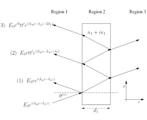
The odd and even layers correspond to glass and air layers, respectively. . . . 35 4.5 Scattering by a slab. . . 41 4.6 Display of the rays considered in Table 4.1 and, in the right bottom graph,

the correction term of equation (4.32). . . 44 4.7 Display of the single reflection arising from thej-th layer for a normal incident

beam. . . 46 4.8 Schematic display of coefficient α_k,p, first realization. . . 46 4.9 Schematic display of coefficient α_k,p, second realization. . . 46

(10)

4.10 Left: Refractive index distribution along a multi-layer structure of thickness 1 mm. Right: Display of the corresponding function |Σ(ξ)|, as defined in equation (4.16), evaluated at 2200 sample positions ξ. . . 47 4.11 Left: Display of|Σ₁(ξ)|evaluated at 2200 sample positionsξ. Right: Difference

between Σ, (obtained by means of equation (4.16)), and Σ₁, obtained by means of equation (4.33), as a function of ξ. . . 48 4.12 Left: Display of|Σ₂(ξ)|, as defined in equation (4.35), evaluated at 2200 sam-

ple positions ξ. Right: Difference between Σ (obtained by means of equation (4.16)) and Σ2 (obtained by means of equation (4.35)) as a function of ξ. . . 49 4.13 Left: Refractive index distribution along a multi-layer structure of thickness

1 mm. Right: Display of Σ(ξ), defined by equation (4.16), evaluated at 2200 sample positions ξ. . . 49 4.14 Left: Display of |Σ₁(ξ)|, as defined by equation (4.33), evaluated at 2200

different positions of the sample. Right: Difference between Σ (obtained by means of equation (4.16)) and Σ₁ as a function ofξ. . . 50 4.15 Left: Display of |Σ₂(ξ)|, as defined by equation (4.35), evaluated at 2200

sample positionsξ. Right: Difference between Σ (obtained by means of equation (4.16)) and Σ2 as a function ofξ . . . 52 5.1 Left: Refractive index distribution. Right: Absorption distribution in blue.

Absorption average in red, κ= 0.9458e−4. . . 58 5.2 Starting point for the scanning process. . . 59 5.3 Absolute value of the correlation function Σ as a function ofξ arising from the

refractive index distribution displayed in Figure 5.1. . . 59 5.4 Left: Coarse sampled first spike in Figure 5.3. Right: Finely sampled first

spike, with circles showing the coarse samples displayed on the left. . . 60 5.5 Left: Coarse sampled second spike in Figure 5.3. Right: Finely sampled second

spike, with red circles showing the coarse samples displayed on the left, and with green circles showing coarse “aliased” samples providing data of very small numerical value, which is prone to be degraded by noise. . . 61 5.6 Mean-square function φ^q=φ^q(n, d). . . 62

(11)

5.7 Mean-square function φ^q =φ^q(n, d): dark reds and dark blues indicate large

and small function values, respectively. . . 63

5.8 Mean-square function φ^q for several values of the refractive index n. . . 64

5.9 Mean-square function φ^q(n, d) as a function ofdfor several values ofn. . . . 65

5.10 Two-layer structure with refractive indexesn₁ and n₂ and thicknessd.. . . . 66

5.11 Blue curve: Given refractive index distribution. Red: solution obtained by means of the minimization procedure detailed in this section. . . 71

6.1 Effect of absorption averaging. Upper left: Prescribed refractive index map. Upper right, lower left and lower right: reconstructions using values κ = 0.6· 10⁻⁴,κ= 0 andκ= 1.2·10⁻⁴ for the average absorption parameter, respectively. 73 6.2 25-layer structure. Upper left: Refractive index distribution. Top right, bottom left and bottom right: Three different (random) absorption distributions. 74 6.3 25-layer structure. Refractive index distribution (blue) and the corresponding reconstruction for three different absorption values distributions. . . 74

6.4 50-layer structure. Upper left: Refractive index distribution. Top right, bottom left and bottom right: Three different (random) absorption distributions. 75 6.5 50-layer structure. Refractive index distribution (blue) and the corresponding reconstruction for three different absorption value distributions. . . 75

6.6 |Σ| for an absorption ranging between 10⁻⁴ and 10⁻³. Top left: 25-layer structure. Top right: 50-layer structure. Bottom left and right: corresponding solutions for these absorption levels. . . 76

6.7 |Σ|for a noise level of the order of 10⁻³ relative to the maximum interference fringe intensity (which is of the order of 10⁻⁵). Top left: 25-layer structure. Top right: 50-layer structure. Bottom left and right: corresponding solutions for these noise levels. . . 77

6.8 Left: Chessboard distribution of the original figure, with original color code. Center: Refractive index assignment. Left: reconstructions under assumption of lenses with numerical aperture of N.A.= 0.054. . . 78

6.9 Same as Figure 6.8. . . 78

6.10 Same as Figure 6.8. . . 79

A.1 The lens. . . 82

(12)

List of Tables

4.1 The functions g(ξ), calculated by direct evaluation of the integral (4.28), and g^trunc(ξ), calculated from a truncated version of equation (4.30), with trunca-

tions as defined in the text. Here n1 = 1.4 andn2 = 1.6;τ = 2(ζ−ξ)/c. . . . 45

4.2 Convergence analysis: exact value Σ = 0.0500432. Here ξ=ζ . . . 45

5.1 Comparison of correlation values in two different bi-layer structures: 1) Layers contain materials of refractive indexesN₁ = 1.4+10⁻⁴iandN₂ = 1.6+5·10⁻⁴i; and 2) Layers containing materials of refractive indexes N3 = 1.4 + 3·10⁻⁴i, N₄= 1.6 + 3·10⁻⁴i, with absorptions equal to the average of the absorptions inN1 and N2. . . 57

5.2 Five-layer structure. . . 67

5.3 Local minima obtained from the minimization process detailed in the text, and displayed by red circles in Figure 5.7. . . 68

5.4 Solution of the inverse problem with κ= 0.9458e−4. . . 70

6.1 Errors in nand dreconstruction. . . 73

6.2 Errors in nand dreconstruction. . . 76

(13)

Chapter 1

Introduction

The problem of imaging material bodies by means of waves and rays has had a tremendous impact on a wide variety of fields, including geology (e.g., providing support for oil and gas exploration as well as enhanced oil recovery operations); medicine (for medical diagnoses and treatment); biology (for anatomical and molecular investigations); military (humanitarian demining, remote sensing); atmospheric science (for evaluation and prediction of weather conditions); and materials science (imaging of solids at atomic length-scales), amongst many others. The imaging techniques used in these fields are manifold; in the biological and medical sciences, for example, we find magnetic resonance imaging, impedance computer tomography, ultrasound, X-ray computer tomography and emission computed tomography.

Using a wide range of sources of lights and sound, the various imaging techniques available provide images at various levels of resolution, literally ranging from hundreds of kilometers in atmospheric applications, to a few microns in some of the most sophisticated biological applications, to a few nanometers in some materials science applications.

In this thesis we are concerned with a new technique, optical coherence tomography (OCT), which has thus far been used for imaging in biology/medical applications. This technique, which is based in interferometry, takes advantage of the low-coherence properties of diode-laser light sources to image selectively (and sequentially) prescribed points within a volumetric sample. Low coherence interferometric microscopes [35, 65] have been successful in producing internal images of thin pieces of biological tissue; typically samples of the order of 1 mm in depth have been imaged, with a resolution of the order of 10 to 20 µm in some portions of the sample. Such images have typically been produced through direct renderings of raw data: the intensities of certain interference fringes as functions of the position of the light-focus within the sample; quite generally, limited post-processing of this data has been

(14)

used.

In this work we address, in a mathematically rigorous manner, the inverse (Maxwell) problem of producing the actual values of the refractive index within a multi-layer sample from given low-coherence interferometric data. Once obtained, such a map of the refractive index variations may be useful in a variety of ways [65]; in particular, a straightforward display of this map yields an image of the internal structure of the sample. The advantages of an approach based on the Maxwell equations are manifold. Notably, such full-wave treatments allow for the consideration of various loss mechanisms such as scattering and absorption in a rigorous manner, and, thus, for production of images that remain faithful throughout the body of the sample. The results of this thesis have been announced in [8].

Our discussion is restricted to one-dimensional configurations; we thus relate our approach to some of the noted one-dimensional inverse problems and inverse-problem solvers for Maxwell’s equations considered previously. As discussed in Section 3.4, existing methods [13, 27, 30] for solution of classical one-dimensional inverse problems for Maxwell’s equation require use of wide wavelength bands, and are thus not applicable to many imaging problems arising in engineering/biological/medical applications. We show, in contrast, that using narrow light-wavelength bands, a certain OCT inverse problem we introduce allows for accurate rendering of refractive index distributions for rather general (thin and pene- trable) samples. We expect that, through use of multiple points of collection of light, the present techniques will extend to cases in which layers are not planar, and, thus, to solution fully three-dimensional low-coherence inverse imaging problems.

1.1 Overview of Chapters

The remainder of this thesis is organized as follows. In Chapter 2 we review the history and development of the fields of microscopy and imaging. In Chapter 3 we discuss the basic elements of the theory of inverse problems, we describe the inverse problems arising in some of the imaging techniques mentioned in Chapter 2, and we present a discussion of previous inverse problem solvers—with emphasis on the previous work on the one-dimensional configurations which form the primary focus of this thesis. In Chapter 4 we focus on the OCT model and we present our strategy for solution of the associated direct problem. We show that, for a multi-layer structure, a rigorous geometrical optics method which takes

(15)

advantage of the coherence properties of OCT light-sources can be used to produce a fast direct-problem solver—as required by our inverse-problem algorithm. In Chapter 5 we then introduce our inverse solver and in Chapter 6, finally, we present a variety of numerical results.

(16)

Chapter 2

Microscopy

2.1 A Brief History of Microscopy

The first useful microscopes were developed in the Netherlands between 1590 and 1608; these first microscopes were simply tubes with lenses at each end. The magnification of these early scopes ranged from 3X to 9X, depending on the size of the diaphragm openings. The lens quality was often poor so the images were not very clear. Antony van Leeuwenhoek (1632- 1723, Holland) built microscopes which gave magnifications up to 270 diameters. With this device he made some of the most important discoveries in biology. He discovered bacteria, sperm cells, blood cells and more. The English chemist, mathematician, physicist, and inventor Robert Hooke confirmed van Leeuwenhoek’s discoveries of the existence of tiny living organisms in a drop of water. Hooke made a copy of Leeuwenhoek’s microscope and then improved upon his design. Later, few major improvements were made until the middle of the 19th century. Present day instruments, changed but little, give magnifications up to 1250 diameters with ordinary light and up to 5000 with blue light. A light microscope, even one with perfect lenses and perfect illumination, cannot be used to distinguish objects that are smaller than half the wavelength of light. Since white light has an average wavelength of 0.55µm, any two lines that are closer together than 0.275µm will be seen as a single line, and any object with a diameter smaller than 0.275 µm will be invisible, or, at best, show up as a blur. To see very small particles under a microscope, scientists must use a different sort of “illumination,” one with a shorter wavelength. In 1934 Ernst Ruska described the construction of an electron microscope which filled the deficiencies of resolution of light microscope. In this kind of microscope, electrons are speeded up in a vacuum until their wavelength is extremely short, only one hundred-thousandth that of white light. Beams

(17)

of these fast-moving electrons are focused on a cell sample and are absorbed or scattered by the cell’s parts so as to form an image on an electron-sensitive photographic plate. If pushed to the limit, electron microscopes can make it possible to view objects as small as the diameter of an atom. Most electron microscopes used to study biological material can

“see” down to about 10 angstroms; although this does not make atoms visible, it does allow researchers to distinguish individual molecules of biological importance. Unfortunately, all electron microscopes suffer from a serious drawback: since no living specimen can survive the needed high vacuum, they cannot show the ever-changing movements that characterize a living cell.

It was Newton’s observations of interference phenomena and Young’s fundamental theory of interference in 1801 that provided the basis of what we know as interference microscope, see [58, p. 9]. In reference [49] Michelson (1852-1931) introduced an interferometer for light reflected from objects. Michelson’s interferometer is the basis of the low-coherence interferometric techniques which underly the OCT microscopes, to whose mathematical study the present thesis is devoted.

2.2 Imaging Techniques

The wide variety of imaging techniques in existence arises from the corresponding diversity of useful energy sources, including light, microwaves, electrons, laser, X rays, ultrasound and nuclear magnetic resonance. The corresponding imaging length-scales range from molecular to geophysical, and the relative advantages and limitations of a given method depends on the way the corresponding energy interacts with the imaged medium. None of these techniques has prevailed over the others, and the selection of a particular one depends on the object to be imaged.

2.2.1 X Rays

R¨ontgen’s discovery [57, p. 2] of X rays in 1895 opened a new era in the practice of medicine:

it allowed visualization into the human body without pain or life-risk. However, X-ray imaging techniques have several important limitations. Small characteristic differences (1%

to 2%) in X-ray attenuation are not detectable. A large percentage of radiation detected is scattered away from the body, thus reducing the signal-to-noise ratio of the recorded

(18)

information. And much detail is lost in the radiographic process due to the superposition of 3-D structural information into a 2-D detector. These problems were minimized with the development of X-ray computed tomography (early 1970s) [57, p. 5].

2.2.1.1 X-ray Computed Tomography (CT)

X-ray CT consists of determining the 2-D or 3-D distribution of tissue attenuation coefficients within the structure by means of mathematical reconstruction techniques based on the Radon inversion formula [57, p. 23]. 2-D images are obtained using a single X-ray tube which rotates 360^◦ recording projections at every angular interval, which may vary between 0.5^◦ to 1^◦. 3-D volume images can be constructed from a sequence of 2-D adjacent images.

The spatial resolution in CT data ranges from 0.1 mm² to 1 mm² while the slice thickness ranges from 1 mm to 10 mm. The CT contrast resolution is in the range of 0.5%.

2.2.2 Magnetic Resonance Imaging (MRI)

Magnetic resonance imaging is an imaging technique used primarily in medical settings to produce high quality images of the inside of the human body [37]. The basic phenomenon of nuclear magnetic resonance has been known since the 1940s and MRI has been developed over the last 60 years. The largest component of the human body—about 75%—is water. A molecule of water (H2O) is composed of two hydrogen (H) atoms and one oxygen (O) atom.

The nucleus of each hydrogen atom consists of a single proton. Under normal conditions, these protons are constantly spinning, which envelopes them within a tiny magnetic field.

Normally, this intrinsic magnetic field is randomly oriented. Under the action of an MRI scanner—which is essentially a very large and powerful magnet—the protons in a body line up either with or against the direction of the scanner’s own strong magnetic field. To make an image, pulses of radiowaves are directed at the area being examined through a special antenna. This knocks the protons off-balance, causing them to flip their orientation.

When the pulse is turned off, the protons return back to their original positions. As they do so, they emit weak radio signals (the MR signal) of a particular frequency, which are analyzed by a computer and combined to create a series of cross-sectional images. 3-D volume images can be acquired using either 2-D multiple adjacent slice techniques or true 3-D volume acquisitions. The spatial resolution in plane ranges from 0.5 mm to 1 mm. MRI contrast is greatest in soft tissue, detecting 5% differences in signals [57, p. 26].

(19)

2.2.3 Confocal Fluorescence Microscopy

In a confocal microscope system, the specimen is not uniformly illuminated throughout its depth. The light is focused on a spot on one volume element of the specimen at a time, and the fluorescent light emitted from this spot is collected by a lens and focused on a pinhole screen blocking light from points out of the focal plane. By scanning many thin sections through the sample, a very clean three-dimensional image of the sample can be built. In practice, the best horizontal resolution of a confocal microscope is about 0.2 µm , and the best vertical resolution is about 0.5 µm. One of the main difficulties of conventional light and fluorescence microscopy experiments is out-of-focus blur degrading the image, reducing image contrast and decreasing the resolution. Out-of-focus information often obscures important structures of interest, particularly in thick specimens. In a conventional microscope setup, not only is the plane of focus illuminated, but much of the specimen above and below this point is also illuminated at the same time. This results in out-of-focus blur from these areas above and below the plane of interest. When living specimens are imaged some serious difficulties may occur: Since the small confocal aperture blocks most of the light emitted by the tissue, including light coming from the plane of focus, the exciting laser must be very bright to allow an adequate signal-to-noise ratio. This bright light causes fluorescent dyes to fade within minutes of continuous scanning (photobleaching). Phototoxicity is also a problem. Excited fluorescent dye molecules generate toxic free-radicals. Thus, one must limit the scanning time or light intensity if one hopes to keep the specimen alive. See http://www.neuro.gatech.edu/potter/2photon.html for more details.

2.2.3.1 Two-Photon Excitation Fluorescence Microscopy

Two-photon microscopy has allowed the possibility of alleviating the problems addressed in Section 2.2.3 [63]; see also http://www.neuro.gatech.edu/potter/2photon.html. In two- photon laser scanning microscopy (TPM), two photons of low energy (half of the wavelength) join forces to excite a fluorophore which would require one photon of twice the energy otherwise. The probability of this to happen is very small and it has quadratic dependence on light intensity. This limits the excitation to a small volume near the aperture and therefore reduces rates for photochemical damage and improved resolution in images of extended samples. The advantages of using lower wavelength results in deeper penetration

(20)

of tissue.

2.2.4 Confocal Scanning Microscopy

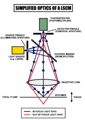
The confocal microscope was invented by Minsky in 1961 [17, 19, 50]. In a confocal microscope, light from a laser is focused by an objective lens to a small spot on the specimen at the focal plane of the lens, see Figure 2.1. Light reflected back from the illuminated spot on the specimen is collected by the objective and is partially reflected by a beam-splitter to be directed at a pinhole placed in front of the detector. This confocal pinhole is what gives the system its confocal property, by rejecting light that did not originate from the focal plane of the microscope objective. Light rays from below the focal plane come to a focus before reaching the detector pinhole, and then they expand out so that most of the rays are physically blocked from reaching the detector by the detector pinhole. In the same way, light reflected from above the focal plane focuses behind the detector pinhole, so that most of that light also hits the edges of the pinhole and is not detected. However, all the light from the focal plane is focused at the detector pinhole and so is detected at the detector. This ability to reject light from above or below the focal plane enables the confocal microscope to perform depth discrimination and optical tomography. A true 3-D image can be processed by taking a series of confocal images at successive planes into the specimen and assembling them in computer memory.

2.2.5 Ultrasound

Ultrasound is sound with a frequency over 20,000 Hz, which is about the upper limit of human hearing. Dussik was the first person to publish information on the medical use of diagnostic ultrasound; see http://www.ob-ultrasound.net/dussikbio.html#hyper. Unlike other techniques reviewed in the present chapter, which involve electromagnetic waves, ultrasound techniques involve longitudinal mechanical waves. In ultrasound, a high frequency sound wave is plunged into the tissue being imaged. The sound waves travel into the tissue or body and are reflected from internal structures with different acoustic properties. Atten- uation of the sound wave may occur with propagation. The time behavior or echo structure of the reflected sound wave is detected and the internal structures are determined from the echo delay [7]. The resolution of ultrasound imaging depends directly on the frequency of the sound waves that are used. Most often sound wave frequencies in clinical applications

(21)

Figure 2.1: Confocal microscopy system.

are in the range of 10 MHz yielding spatial resolution up of 150µm. Resolution of the order of 15-20 µm was reached using much higher frequencies with the disadvantage that, since high frequencies are strongly attenuated for most biological tissue, this imaging is limited to depth of a few millimeters. On the other hand, frequencies in the range of 10 MHz are easily transmitted, allowing high penetration in tissue up to several tens of centimeters deep within the body. Use of ultrasound is not limited to medical applications: ultrasound techniques have important industrial applications. For instance, ultrasound is used to measure the viscosity and temperature of molten materials at very high temperatures, or to obtain concentration measurements, and ultrasonic mass flow measurement. [5, 20, 55]

2.2.6 Optical Coherence Tomography (OCT)

We can find the basis of what we know as interference microscope in Newton’s observations of interference phenomena and Young’s fundamental theory of interference [58, p. 10]. The earliest applications of low-coherence interferometric techniques were related to the detec- tion of faults within fiber-optical cables and network components using optical-coherence domain reflectometry [28, 64, 68], but soon the technique found application in medical and

(22)

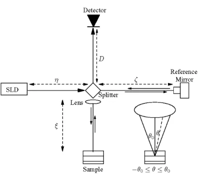
biological fields [34, 38, 60]. The basis of a low coherence interferometric microscope is a Michelson interferometer with a low-coherence light source (a super-luminescent diode). In an OCT microscope, 1) The sample to be imaged is placed in one arm of the interferometer, see Figure 4.2, and, 2) The light from the reference mirror (which is positioned at variable distances) and the light from the sample are correlated and detected. Since a light source of low coherence is used, the detector only responds to interferometric intensity fluctuations when the sample and the reference reflection have traveled through approximately the same optical lengths, thus giving information on the character of the scatterer to be found in a given position within the sample. Previous approaches to OCT imaging were based on rendering of the raw interference intensity maps to produce an image of internal structure of the sample. A detailed description of OCT tomography is presented in Chapter 4.

Additional information concerning the techniques described in the present Chapter 2 can be found in [7, 16, 17, 57–59].

(23)

Chapter 3

Inverse Problems

3.1 Introduction

Some of the most important mathematical problems arising in the imaging field belong to the general class of inverse problems. To preface our introductory history of inverse problems, I would like to bring to these pages the words of Reese T. Prosser in his review [54] of the bookMultidimensional Inverse Scattering Problems by Alexander G. Ramm:

“The first postwar discussion of a recognizable inverse problem, in 1946, is due to Borg [6], who was concerned with the problem of recovering the density function for a one-dimensional vibrating string from a knowledge of its eigenfrequencies and eigenweights. Shortly thereafter there arose a considerable interest in determining the shape of certain nuclear potentials in quantum mechanics from measurements obtained from the scattering of elementary particle wave functions by these potentials. In 1949 Levinson [46] showed that the potential function which scatters a one dimensional particle is uniquely determined by the asymptotic phase of the particle wave function. In 1952 Jost and Kohn [42] gave a simple algorithm for constructing the potential function from the asymptotic phase.

Meanwhile, in 1951 Gelfand and Levitan [27] produced a general method for recovering the potential function in the one-dimensional Schr¨odinger equation from the spectral data, and Marchenko [2] extended the method to include recovering the potential directly from the scattering data. All these attempts took on a renewed interest in the 1960s, when it was discovered by Gardner, Greene, Kruskal, and Miura [26] that the direct problem for the nonlinear Korteweg- deVries equation could be completely resolved by first resolving an associated

(24)

inverse problem for the linear Schrödinger equation. The inverse problem for the Schrödinger equation then took on all the aspects of a thriving cottage in- dustry. The extension of these results to the more realistic and more interesting cases in higher dimensions has not come easily. The difficulties are all present in the prototype problem of the scattering in three dimensions of an elementary particle by a scalar potential. Mathematically, the problem can be briefly stated this way: Consider the time-independent Schrödinger equation

∇u(x) +k²u(x)−q(x)u(x) = 0;x∈R³.

This equation governs the scattering in three dimensions of the quantum mechanical wave function u(x) by the potential q(x). The relevant solution u(x) satisfies the associated integral equation

u(x, k) = exp(ix·k)− Z

R³

exp(i|k||x−y|)

4|x−y| q(y)u(y, k)dy.

As|x| → ∞, this solution has the asymptotic form u(x, k) =e^ik·x−T(k⁰, k)e^ikr

4πr +O(1/r),

This form may be interpreted physically as consisting of an ingoing plane wave plus an outgoing spherical wave weighted by the “T-matrix”

T(k⁰, k) = 1 4π

Z

R³

e^−ik⁰^·yq(y)u(y, k)dy,

which embodies the measurable scattering information. Here k is the ingoing plane wave vector andk⁰ is the outgoing scattered wave vector, withr=|x|and k=|k|=|k⁰|. Writingθ=k/|k|,θ⁰ =k⁰/|k⁰|, and A(θ⁰, θ, k) =T(k⁰, k), we can state the relevant three-dimensional scattering problems as follows:

• The direct potential scattering problem: Givenq(x), findA(θ⁰, θ, k).

• The inverse potential scattering problem: GivenA(θ⁰, θ, k), findq(x).

The inverse potential scattering problem breaks naturally into several pieces:

(25)

• The uniqueness problem: GivenA(θ⁰, θ, k), show that at most one potential q(x) can give rise toA(θ⁰, θ, k).

• The characterization problem: Given A(θ⁰, θ, k), find conditions which guarantee that at least one potential q(x) can give rise to A(θ⁰, θ, k).

• The existence problem: Given A(θ⁰, θ, k), show that at least one potential can give rise to A(θ⁰, θ, k).

• The stability problem: Show that small changes in the data A(θ⁰, θ, k) result in small changes in the potentialq(x).

• The reconstruction problem: Given A(θ⁰, θ, k), construct, analytically or numerically, at least one potential giving rise toA(θ⁰, θ, k).

• The partial data problem: Given some portion of A(θ⁰, θ, k), construct at least one potentialq(x) giving rise to that portion ofA(θ⁰, θ, k).

None of these problems is easy, and most are still open.”

In Chapter 3.2 below we present a brief introduction to the main techniques generally used in the solution of inverse problems; in Chapter 3.3 we then provide a succinct description of the types of inverse problems arising in the fields biological, medicine and engineering.

3.2 Inversion Methods

Given an operatorL_λ depending on the parameter λand the equation

L_λu=f, (3.1)

we refer to the forward problem as the problem to solve uin (3.1) for a given λand f [48].

Now, if we are given an OperatorB such that

Bu=g, (3.2)

then we refer to an inverse problem as the problem of finding λfrom the system of equations (3.1) and (3.2) for given f and g.

(26)

As it happens, inverse problems are often “ill-posed”. To define the concept of ill- posedness let A be a general map from a Hilbert space X into a Hilbert space Y. Then, the equation

Ax=b (3.3)

is called well-posed if

1. the equation is solvable for each b,

2. the solutionx is uniquely determined, and 3. the solutionx depends continuously onb.

Otherwise, the equation is said to be ill-posed.

Most imaging problems are ill-posed. They commonly fail to satisfy condition (3) , which leads to instability, i.e., a small data error δ in b can lead to a large error in the computed solution x. Knowledge of information about the functionx such as smoothness and size might be used to enhance the stability of the problem. Denoting by b^δ =b+δ, a regularization method is any method that computes fromb^δ and from a knowledge of a set M ⊆X where the solution must lie, an element x^δ ∈ M such that kx−x^δk ≤ (δ) with (δ)→0 asδ →0. Following [48], we summarize some common regularization methods

1. The Tikhonov-Phillips Method

2. The Truncated Singular Value Decomposition 3. Iterative Methods

4. Regularization by Discretization 5. Maximum Entropy

3.2.1 The Tikhonov-Phillips Method

This regularization method [66] seeks the minimizer x^δ of minx∈X

n

kAx−b^δk_Y +αkxk_Xo ,

(27)

whereα >0 is a suitably chosen “regularization parameter.” If the operatorAis linear [52], then

x^δ= (A^∗A+αI)⁻¹A^∗b,

whereA^∗is the adjoint ofA. Application of this technique in medical imaging can be found in [51, 53, 56]. Other applications of this technique can be found such as to determine the particle size distribution of latex [23] or to estimate the relaxation spectrum of viscoelastic materials [22].

3.2.2 The Truncated Singular Value Decomposition

The idea of this technique consists of expressing the approximate solution x^δ by

x^δ = X

k,σk≥σ

1 σ_k

b^δ, b_k

x_k,

wherex_k,b_k are orthonormal systems inX,Y, respectively, and σ_k are the singular values of the operator A and its adjointA^∗, i.e,

Ax=

∞

X

k=1

σ_k(x, x_k)b_k,

A^∗x=

∞

X

k=1

σ_k(b, b_k)x_k.

As pointed out in [47], the decay of the singular valuesσ_k is a measure for the ill-posedness of the operator. In most cases this technique is too expensive to provide an efficient practical reconstruction method, but on the other hand, it is a very valuable tool for analysis. An example of the application of this technique can be found in [61].

3.2.3 Iterative Methods

The term “iterative method” refers to a wide range of techniques that use successive approximations to obtain more accurate solutions to a linear system at each step. Iterative methods act as regularization if the iteration is stopped early enough. As indicated in [47], iterative methods compute first the contributions to large singular values and thus, the smoother part of the solution. Iterative techniques that seek to minimize the defect ||Af −g|| with respect to f can be used in the nonlinear context as well, and, thus, such methods can be

(28)

applied to the (typically nonlinear) imaging problems [47]. With a finite set of datag∈R^M and f ∈R^N we write

φ(f) = 1 2

M

X

m=1

F_m², (3.4)

where Fm = [(Af)m−gm], and (for sufficiently smooth operators A :R^N → R^M) expand it in the form

φ(f +v) =v· ∇φ(f) + 1

2v·H(f)v+ (||v||³), (3.5) where∇φ(f) =JA(f)^TF,JA(f)mn= (∂(Af)m/∂fn) is the Jacobian matrix of the operator A and where, defining for a given functionh(~x),

∇²h

ij = (∂²h/∂x_i∂x_j), we have set H(f) =J_A(f)^TJ_A(f) +

M

X

m

(Af −g)_m∇²(Af)_m.

Seeking minimization of the second order approximation by means of Newton’s methods we obtain the algorithm

f_k+1=f_k+v^k, (3.6)

wherev^k is the solution of the system

H(f^k)v^k=−∇φ(f^k). (3.7) To avoid evaluation of second derivatives one can approximate the Hessian (3.7) byH(f)≈ φ^0Tφ⁰ arguing that F is sufficiently small near the solution. The Newton-type method resulting from this simplification is referred to as the “Gauss-Newton” method; see also [11]

and Section 5.3. Examples of iterative methods applied to imaging techniques can be found in [45].

3.2.4 Regularization by Discretization

This method of regularization [48] consists of approximating the operator A in (3.3) by a discretizationAh of A with step-size h in such a way that if h→ 0 then Ah → A in some sense. SinceA⁻¹ is not continuous, the solutiong_h of the equation

f_h =A⁻¹_h g_h, (3.8)

(29)

will not converge to a good approximation of the solution f when the procedure is applied tog^δ. However, with a suitable election of h=h(δ)

f^δ =A⁻¹_h(δ)g_h(δ), (3.9)

may be made to satisfy||f−f^δ||< (δ). Often the discretization is performed by projecting on finite dimensional subspaces. Applications of this technique to problems of medical imaging can be found in [4].

3.2.5 Maximum Entropy

This method searches for minimizersf_δ of the problem minf∈X

nkAf −g^δk_Y +αΩ(f)o ,

where Ω(f) is given by

Ω(f) =− Z

f(x) log|f(x)|dx.

The minimization problem is then solved by means of iterative methods. This is applied for example in positron-emission tomography, see [33].

3.3 Inverse Problems Arising in the Imaging Field

3.3.1 X-Ray CT - Radon Transform

To describe the CT imaging problem, let us consider a domain Ω ∈ R² and the linear attenuation coefficient a(x, y) defined on Ω. If I0 is the intensity of the source and I the intensity transmitted along the rayL, then

I =I₀e⁻^R^L^a(x,y)dL. (3.10)

The mathematical problem in transmission tomography is to determine a from measurements of I for a large set of rays L [48]. If L is the straight line connecting the source

(30)

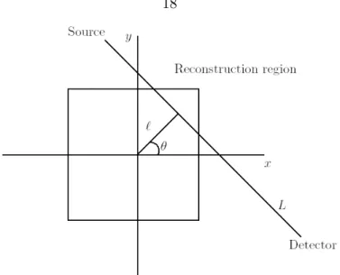
Figure 3.1: Data collection for CT.

X0= (x0, y0) and the detectorX1= (x1, y1), then we have log

I I₀

=− Z 1

0

a((X0−X1)s+X0)ds, (3.11) which is a reparametrization of the Radon Transform R defined by [32]

[Rˆa](`, θ) = Z ∞

−∞

ˆ a(p

`²+z², θ+ tan⁻¹(z/`))dz), (3.12) where ˆa(r, φ) =a(rcosφ, rsinφ) is the attenuation coefficient in polar coordinates. Here` denotes the distance of the straight line L to the origin of coordinates and θ denotes the angle that the perpendicular toL forms with the positivex axis, see Figure 3.1.

The input data to a reconstruction algorithm are estimates of the values of [Rˆa](`, θ) for a finite number of pairs (`, θ); its output is an estimate of ˆa. The inverse operator for the Radon Transform we are looking for is given by

[R⁻¹p](r, φ) = 1 2π²

Z π 0

Z E

−E

1

rcos(θ−φ)−`

∂p(`, θ)

∂` d`dθ, (3.13)

wherep(`, θ) = 0 if |`|< E. It is important to note that for the reconstruction problem we need a discrete version for this inverse operator, see [32].

(31)

3.3.2 Ultrasound Computed Tomography

Consider an object Ω with refractive index n which is probed by a plane wave with wavelength λand wave number k= 2π/λ, uθ =e^ikx·θ, traveling in the direction given by the unit vector θ. The total fieldu(x) =u(x, θ) satisfies the Helmholtz equation

∇u+k²(1 +m)u= 0, m=n²−1,

and the scattered field u−u_θ satisfies radiation condition at infinity. The inverse problem to be solved is as follows: Given

u(x, θ), θ∈S²

forx on a certain surface outside Ω, determine mwithin Ω.

Most solvers for this problem are based on linearization, such as those given by the Born and Rytov approximations [48]. The Born approximation assumes that the field inside the body can be approximated by the incident field and leads to the linear integral equation

u(x, θ) =u_θ−k² Z

Ω

G(x−y)m(y)dy, x /∈Ω (3.14) form, where Gis the 3 dimensional Green function

G(x) = e^ik|x|

4π|x|.

Unfortunately, the assumptions underlying the Born and Rytov approximations are not satisfied in medical imaging since they do not take into account multiple reflections events which are of considerable relevance in scattering from biological tissues. Thus, the reconstructions ofmobtained from solving the integral equation (3.14) can be of relatively poor quality [48, p. 96].

3.3.3 Optical Tomography

Optical tomography is an imaging technique which seeks to recover the spatial distribution of tissue absorption and scattering parameters in the near-infrared and optical wavelength range from surface measurements of light transmission [48]. The process is described by the

(32)

(Boltzman) transport equation

∂u(x, θ, t)

∂t +θ.∇u(x, θ, t) +a(x)u(x, θ, t) =b(x) Z

S²

η(θ·θ⁰)u(x, θ⁰, t)dθ⁰+f(x, θ, t) for the density u(x, θ, t) of photons at x∈Ω flying in the direction θ ∈S² at time t. The constants a and b are tissue parameters. The scattering kernel η is assumed to be known and f is the source term. The initial and boundary conditions are given by

u(x, θ,0) = 0 in Ω×S²

u(x, θ, t) = 0 on ∂Ω×S²×R, ν_x·θ≤0.

The inverse problem arising from this model seeks to determine the tissue parametersaand bfrom a given outward radiation

g(x, θ, t) =u(x, θ, t) on ∂Ω×S²×R, ν_x·θ≥0.

Some of the best-known numerical methods for the solution of this inverse problem are of iterative type, where iterations are either applied directly to the transport equation or to its so-called diffusion approximation—which is an approximation to the transport equation by a parabolic differential equation. Unfortunately the inverse problems for equations of this type are very ill-posed. An extensive review of the methods developed to solve the transport inverse problem can be found in the references [3] and [4]. A study of the advantages of incorporating prior information to the reconstruction process is given in [62]. Quasi-Newton methods to the solution of the inverse problem are studied in [45].

3.4 1-D Inverse Problem for the Helmholtz Equation

The Helmholtz equation governs a variety of physical phenomena related to propagation of acoustic and electromagnetic waves [14, 44], and, it has thus come to be a centerpiece in a wide range of fields, including as medical diagnostics, non-destructive industrial testing, anti-submarine warfare, oil exploration, etc. [13]. As is well known, the inverse problem for the Helmholtz equation is highly nonlinear. In the one dimensional case, the problem can be reduced to a linear one, but the procedure is not stable numerically [27]. In this section

(33)

we present some of the inverse scattering solvers proposed previously for inverse problems associated with the Helmholtz equation

u⁰⁰+k²n(x)²u= 0, (3.15)

and the closely related Schr¨odinger equation

u⁰⁰+k²u=V(r)u. (3.16)

The scattering of a particle of energy E=k² by a central potentialV(r) (a function of r=|~r|)) is governed by the three dimensional Schr¨odinger equation

∆u(~r) +Eu(~r) =V(r)u(~r), (3.17) which can be reduced to a sequence of one-dimensional (radial) Schr¨odinger equations expressing the solutionu in terms of its spherical harmonics expansion,

ϕ⁰⁰_l +

E−l(l+ 1) r²

ϕl=V(r)ϕl, (3.18)

The problem of determiningV(r) from scattering data has been the subject of very extensive studies. In what follows we discuss briefly the contributions introduced in [13, 27, 30].

Gelfand-Levitan method. In [27] the authors dealt with the problem of determining the potentialV(x) in the second order differential equation

y⁰⁰+ (E−V(x))y= 0, (3.19)

(defined on the interval (0,∞) with initial conditions y(0) = 1, y⁰(0) = h and under the assumption that V(x) is continuous) from a given spectral function ρ(E) and the corresponding bound states. The spectral function ρ(E) is a monotonic function, bounded on each interval, such that for any function f(x) with integrable square the equation

Z ∞ 0

f²(x)dx= Z ∞

−∞

fb(E)²dρ(E)

(34)

holds, where

fb(E) = Z ∞

0

f(x)φ(x, E)dx,

and where φ(x, E) is the solution of equation (3.19) with the given boundary conditions.

The bound states correspond to the solutions of (3.18) which satisfy the boundary conditions ϕ(E,0) = 0, ϕ⁰(E,0) = 1 and are square-integrable on the whole positive real axis.

The authors gave conditions ensuring the existence of a potential V that gives rise to a prescribed spectral function ρ, and they provided a method to compute V(x) and h for a given admissible ρ. To do this the authors reduced the inverse problem to solution of a linear integral equation

g(x, y) + Z x

0

K(x, t)g(x, t)dt+K(x, y) = 0, where

g(x, y) = Z ∞

−∞

cos(√

Ex) cos(√

Ey)dσ(E),

and

σ(E) =







ρ(E)− ²_π√

E, E ≥0, ρ(E) E <0.

Once the function K is known, the potential V(x) and the initial condition h can be obtained:

V(x) = 2dK(x, x) dx and h=K(0,0).

We emphasize that the spectral function is related to the phase-shift δ0 of the wave function ϕ₀ and which is a function of the energy E and which is a measurable quantity.

Thus, from knowledge ofδ0it is possible to obtainρ(E) and then, following the steps detailed above, to determine the potential V. A more detailed description of this method is given in [12]. Marchenko modified the theory of Gelfand and Levitan making it possible to obtain the potentialV(x) directly from scattering data. Indeed, denotingS(k) = exp(2iδ(k)) and

A₀(t) = (2iπ)⁻¹ Z ∞

−∞

[S(k)−1]e^iktdk,

(35)

Marchenko obtained a linear integral equation A(r, t) =A₀(r+t) +

Z ∞ r

A(r, s)A₀(s+t)ds, t > r, from whose solution it is possible to obtain the potentialV:

V(r) =−2dA(r, r) dr .

It is possible to prove that Marchenko’s theory is equivalent to Gelfand-Levitan’ s theory;

see [12, p. 73].

Integral equation method. In reference [30] the author deals with an inverse problem of the form

y⁰⁰(x) + ω²

v(x)²y(x) = 0 y⁰(0) + iω

v(0)y(0) = 2iω (3.20)

y⁰(1)− iω

v(1)y(1) = 0,

where the goal is to determine the unknown velocity v from data of the scattering field prescribed at a set ofωvalues. The procedure is the following: After the change of variables

τ = Z x

0

v(s)⁻¹ds,

a new formulation of the problem is obtained:

u⁰ c

0

+ω²u

c = Lu= 0 u⁰+iωu

(0) = 2iω u⁰−iωu

(1) = 0,

where u(τ) =y(x(τ)) and c(τ) =v(x(τ)). Then, noting that the operatorL depends on c explicitly the problem can be expressed as the integral equation forc:

Z 1 0

uLu_i = Z 1

0

(u_i+u_s)Lu_i =−2iωu_s(0;ω), (3.21)

(36)

where u_s =u−u_i. The values of u_s(0;ω) for the set of ω_j =jπ/2 = k_j/2 are our known data. The most general approach to obtain a solution of equation (3.21) considers the operatorL₀v=v⁰⁰+ω²v= 0 andu_i=e^iωτ and thus, equation (3.21) can be written as

Z 1 0

e^iωτ iωe^iωτ +u⁰_s

γ(τ)dτ = 2iωu_s(0;ω), (3.22) whereγ =c⁰/c or

iω Z 1

0

e^2iωτγ(τ)dτ = 2iωu_s(0;ω)− Z 1

0

γ(τ)u_s(τ, w)e^iωτdτ. (3.23) Now, assuming thatc⁰(0) =c⁰(1) = 0 so that the sine series of γ is appropriate, dividing by iω, taking the imaginary part and setting the set ω=ω_k =kπ/2 the author gets

Z 1 0

γsinkπτ dτ = 2Im(u_s(0;ω_k)) + 1 ω_kRe

Z 1 0

γu⁰_s(τ;ω)e^{ikπτ /2}dτ

=B_k/2, (3.24) whereB_k represents the coefficients in

γ(τ) =

∞

X

1

Bksinkπτ.

Note that theB_k are not directly available since the integral in the right hand side involves the unknown γ. The author uses iteration to tackle this problem. First, he considers equation (3.24) without the integral term, i.e.,

Z 1 0

γsinkπτ dτ = 2Im(u_s(0;ω_k)), and he obtains

γ0(τ) = 4

N

X

1

Im(us(0;ωk) sinkπτ), (3.25)

c0(τ) = exp 4 π

N

X

1

Im(us(0;ω_k)) (1−coskπτ)/k

!

. (3.26)

(37)

Then using (3.25) and (3.26) in (3.24) it is possible to compute B_k and thus obtain a new γ and a newcby means of

γ(τ) =

N

X

1

B_ksinkπτ,

c(τ) = exp 1 π

N

X

1

B_k(1−coskπτ)/k

! .

This process is continued to convergence.

Spline projection method. In the article [18] the authors seek an approximation to the function n(x) such that, given the reflection coefficient R(ω) of the corresponding layered structure, the solution u(x) of the boundary value problem

u⁰⁰(x) +ω²n(x)²u(x) = 0

u⁰(0) +iωn0(0)u(0) = 2in0ω (3.27) u⁰(1)−iωn₀(1)u(1) = 0,

satisfies u(0) = 1 +R(ω) and u⁰(0) = in0ω(1−R(ω)) for all values of ω. The method, which assumes knowledge of a discrete set of values of R(ω), proceeds by approximating n(x) using ak-th order spline expansion of the form

n(x)≈n(x) =¯

N

X

i

λ_iB_i,k(x).

This expansion leads to the solution of a non-linear system of equations in λi, which is solved by means of Levenberg-Marquardt algorithm. The authors show that this technique gives a certain degree of stability when sufficiently small noise errors are present in the measured data.

Techniques based on trace formulae. Trace formulae methods were introduced in reference [15] to study one-dimensional inverse quantum mechanical scattering problems in the line. In reference [13] the authors introduced trace formulae different from those of [15];

in what follows we discuss briefly the approach [13], which is more closely related than [15]

to the imaging problems considered in this thesis.

(38)

In reference [13] the authors deal with the inverse problem for the one-dimensional scalar Helmholtz equation for electromagnetic scattering by a layered structure described by a (continuous or discontinuous) functionq =q(x):

φ⁰⁰(x, k) +k²(1 +q(x))φ(x, k) = 0. (3.28) To describe this inverse problem in detail, for each complex k ∈C⁺ (= complex numbers with positive imaginary part) we consider the functionsφ+(x, k) (total field for left-to-right incidence) andφ−(x, k) (total field for right-to-left incidence) given by

φ₊(x, k) = φ_inc+(x, k) +φ_scatt+(x, k) (3.29) φ−(x, k) = φinc−(x, k) +φscatt−(x, k),

where

φinc+(x, k) = e^ikx (3.30)

φinc−(x, k) = e^−ikx,

and φscatt+(x, k), φscatt−(x, k) satisfy the Helmholtz equation and the outgoing radiation boundary conditions

φ⁰_scatt(0, k) +ikφ_scatt(0, k) = 0 (3.31)

φ⁰_scatt(1, k) +ikφ_scatt(1, k) = 0, respectively. Defining for k∈C⁺ the impedance functions

p+(x, k) = φ⁰₊(x, k) ikφ+(x, k) p−(x, k) = φ⁰₋(x, k)

−ikφ−(x, k), (3.32)

the inverse problem under consideration is described as follows: given the valuesp₊(0, k) of the impedance function at x= 0 for a finite number of frequencieskj =jh, j = 1,2, ...., N (where h is a positive constant), produce an approximation of the potential q(x) in the interval [0,1].

(39)

In order to solve this problem the authors obtain the trace formulae q⁰(x) = 2

π(1 +q(x)) Z ∞

−∞

(p₊(x, k)−p−(x, k))dk

≈ 2

π(1 +q(x)) Z kmax

−k_max

(p₊(x, k)−p−(x, k))dk, (3.33) and the Riccati equations

p⁰₊(x, k) = −ik(p²₊(x, k)−(1 +q(x)), p⁰₋(x, k) = ik(p²₋(x, k)−(1 +q(x)), with initial conditions

p⁰₊(0, k) = p0(k), p⁰₋(0, k) = 1,

q(0) = 0.

This is an integro-differential system of equations for p+, p− and q, which, as it is shown in [13], admits a unique solution for for sufficiently large values of k_max. Further, this solution is stable with respect to small perturbations of the initial data p0(k).

In order to implement the algorithm it is necessary to select appropriate values for the truncation parameter kmax in equation (3.33); the authors use values ranging in the interval 5 ≤ k_max ≤ 100 and they perform the integration using N_k integration points (wavenumbers) with 50≤Nk≤3200.

Applicability of previous Helmholtz inverse solvers to imaging problems. The inverse solvers described above in this section require knowledge of data in a wide frequency (energy) range, a requirement which may render them inapplicable to some of the most important engineering/medical configurations arising in practice. Indeed, the algorithm [13]

described in the previous subsection, for example, uses values of the truncation parameter k_maxof equation (3.33) in the range 5≤k_max≤100 with wavenumber steps 0.1≤h_k≤0.2 for kmax = 5 and h_k = 0.1 for kmax = 100. Even in the most favorable case, kmax = 5 andh_k= 0.2, we would have an infinite ratio of maximum to minimum wave number (if an

(40)

integration scheme centered at zero is used), or a ratio of 5/0.1 = 50—if the infinite ratio is avoided by integrating between, say,−4.9 and 5.1 with the same step hk = 0.2. Thus, in the best possible scenario considered in [13] there is a factor of 50 between the lowest and largest wavenumbers used, and, thus, a corresponding factor of 50 between the largest and smallest wavelengths used. For the values k_max = 100 and h_k = 0.1 used in [13], in turn, the largest wavelength ratio is 100/0.05 = 2000.

As is well known, unfortunately, both the absorption and the refractive index of materials depend very strongly on wavelength; the variation of these quantities for water, for example, is depicted in Figure 3.2. It is easy to see from this figure that, for imaging of biological bodies—in which water is a main component— for example, an inverse problem solver must only rely upon a range of frequencies restricted to the narrow wavelength band around the visible band—for which the absorption is very small, and for which the index of refraction is virtually constant. Indeed, use of light outside this narrow band (for which the combined effects of the orders-of-magnitude larger absorption losses and the uncertainties caused by the fast and large variations of the refractive indexes—which, in view of Figure 3.2 are certain to occur, but which, because of the presence of other materials in combination with water, are actually unknown), cannot provide any useful information about the internal structure of a water-based sample.

Clearly, the range of frequencies required by the algorithm of [13], in which the ratio of smallest to largest frequency is of the order of 50, cannot all be accommodated within any acceptable neighborhood of the 0.4-0.75 µm visible band—nor within any region R of the spectrum satisfying the following three fundamental premises:

• R contains sufficiently short wavelengths—to resolve relevant features,

• Frequencies inR give rise to sufficiently small absorption—for adequate penetration, and

• Frequencies inR give rise to negligible refractive index variations for all of the materials making up the sample—without which the inverse problem is not determined.

Examination of tables of optical constants of materials [1, 43] suggests that, for most engineering/medical/biological configurations, involving e.g. water, semi-conductors, metals, glass, silicon, etc., the required set of three premises mentioned above is not satisfied in

(41)

Figure 3.2: The index of refraction (top) and absorption coefficient (bottom) for liquid water as a function of linear frequency [40]. The visible region of the frequency spectrum is indicated by the vertical dashed lines. The absorption coefficient for sea water is indicated by the dashed diagonal line at the left. Note the logarithmic scale in both directions.