Spin-Bose metal and SU(2)-invariant Majorana spin liquids

However, the experiment reports no observation of the thermal Hall effect due to deconfined spinons [23]. In the remainder of this chapter, we summarize the experimental evidence on the state of spin liquids in κ-(ET)2Cu2(CN)3 in Chapter 1.1 and EtMe3Sb[Pd(dmit)2]2 in Chapter 1.2.

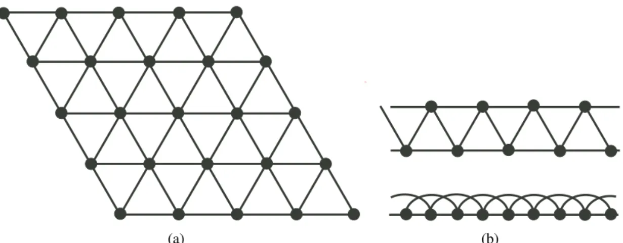
Figure 1.1: Schematic pictures of antiferromagnetic Ising spin model on a square and a triangle

Hence, the ET dimers in (b) can be simplified to the triangular lattice model with each site occupied by exactly one electron. We note that due to the small charge gap, the theoretical quantum spin model must include the high-order spin interactions (i.e., 3-site or 4-site ring exchange terms) in addition to the usual Heisenberg interactions.

The solid lines represent the results of the series expansion of the triangular lattice Heisenberg model. b) 1H NMR spectra of κ-(ET)2Cu2(CN)3 (left) and κ-(ET)2Cu(CN)2Cl (right) single crystals under magnetic fields acting perpendicular to the conductive layer. The result indicates the first realization of a quantum spin liquid in κ-(ET)2Cu2(CN)3 due to strong spin frustration on a nearly equilateral triangular lattice.

Figure 1.4: Adopted from [26]. (a) Temperature dependences of spin susceptibilities of κ- κ-(ET) 2 Cu 2 (CN) 3 and κ-(ET) 2 Cu(CN) 2 Cl

Gapless spin liquid material: EtMe 3 Sb[Pd(dmit) 2 ] 2

Crystal and electronic structures of EtMe 3 Sb[Pd(dmit) 2 ] 2

The intradimer linkages are much stronger than the interdimer linkages and thus each dimer can be treated as a single unit and ultimately simplified to the triangular lattice model with three unequal transfer integrals, t, t0 and t00. According to calculations from quantum chemistry, t0/t'0.92 for EtMe3Sb[Pd(dmit)2]2 is so frustrated that a spin-liquid phase can be realized.

Spin liquid in EtMe 3 Sb[Pd(dmit) 2 ] 2

The inset shows the temperature dependence of the stretching exponent (β). b) Low temperature heat capacity (Cp) for EtMe3Sb[Pd(dmit)2]2 and Et2Me2Sb salt. Such a field dependence of the thermal conductivity of EtMe3Sb[Pd(dmit)2]2 is likely to provide information of the field-induced phase excitation, but not the intrinsic properties of the fully gapless spin liq.

Figure 1.7: Adopted from [26]. (a) Temperature dependence of the spin susceptibility of randomly oriented samples of EtMe 3 Sb[Pd(dmit) 2 ] 2

Overview of thesis

Let us now express the bosonized Hamiltonian density in terms of the chiral boson field. Under bosonization, the two chiral terms of the "quadratic" form become proportional to (∂xφP)2 and can be treated to renormalize the Fermi velocity in Eq.

Figure 2.1: (a) Noninteracting electrons hop on the 1D chain with nearest-neighbor hopping amplitude t

Weak-coupling renormalization group (RG) and current algebra

After expansion in terms of continuum fermions, the allowed four-fermion interactions are strongly limited by the symmetries of the system. In principle, if we consider any product of current operators, the operator products can be treated qualitatively as some generalized Wick contractions.

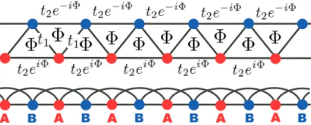
Spin Bose-metal theory on the zigzag strip

SBM via Bosonization of gauge theory

In this (1+1)D continuum theory, we work in scale, eliminating the spatial components of the scale field. In the gauge theory analysis, we cannot determine the mean value θ(0)ρ+, which is important for the detailed properties of the SBM.

SBM by Bosonizing interacting electrons

We know that in this case even an arbitrary weak repulsive interaction will induce an allowed four-fermion Umklapp term that will be marginally important and drive the system into a 1D Mott insulator. As in the single-band case, Umklapp terms are needed to drive the system into a Mott insulator.

Fixed-point theory of the SBM phase

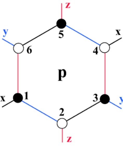
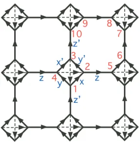
Note that there are three types of links (x, y, and z links in different colors) on the honeycomb grid. b) Graphical visualization of Majorana representation on the honeycomb lattice.

Original Kitaev model on the honeycomb lattice

Setup for two-band electron system
Weak coupling renormalization group
Fixed point for stable C2S2 phase
Numerical studies of the flows
Examples of phase diagrams with C2S2 metal stabilized by ex-

Weak coupling phase diagram for potential Eq. (3.31)
Weak coupling phase diagram for potential Eq. (3.31)

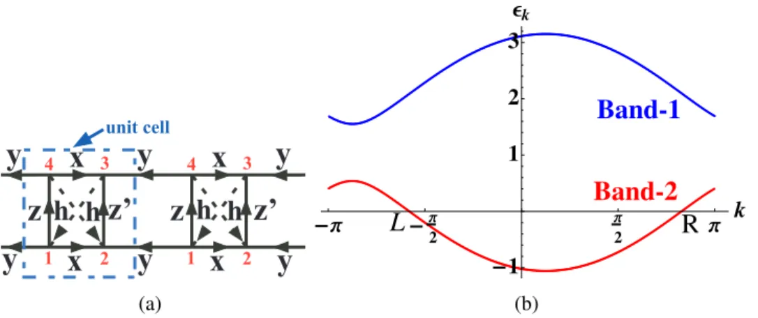
Due to such symmetry, only half of the degrees of freedom in the Majorana Hamiltonian are physical. The spectrum of the gapless phase in the Brillouin zone contains two Dirac cones (more precisely, two half-Dirac cones since only half of the degrees of freedom are physical).

Figure 2.5: The W p is defined around the lattice plaquette (i.e., hexagons) and p is a label of the plaquette.

Weak-to-intermediate coupling: Phases out of C2S2 upon increasing inter-

Harmonic description of the C2S2 phase

The fixed point matrix elements will differ somewhat from the bare values above, but we ignore this in our coarse analysis of the intermediate coupling regime. We thus have a precise parallel with the weak coupling analysis of the C2S2 fixed point in chapter 3.1.

Mott insulator driven by Umklapp interaction. Intermediate cou-

Instability out of C1[ρ−]S2 driven by spin-charge cou-
Instability out of C1[ρ+]S0 driven by Umklapp H 8

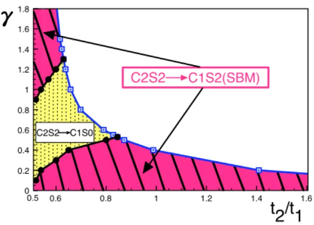
With these remarks in mind, we now describe how we analyze stepwise eliminations from C1[ρ−]S2 and C1[ρ+]S0 in the same procedure. In this analysis, focusing on the "ρ+" and "ρ−" fields, we can also roughly estimate the extent of C1S2 or C1S0 phases when either of them emerges from C2S2.

Numerical results

Intermediate coupling phase diagram for model with po-
Intermediate coupling phase diagram for model with po-

Here, the horizontal interval is equal to the extent of the C2S2 phase in the weak coupling analysis from Fig. More realistically, we expect the C2S2 phase to peak somewhere in the middle of the range shown in Fig.

Figure 3.6: Projection of phases obtained out of the C2S2 of Fig. 3.4 as we increase overall repulsion strength V , which we imagine to be the z-axis perpendicular to the page (Fig

Summary and discussion

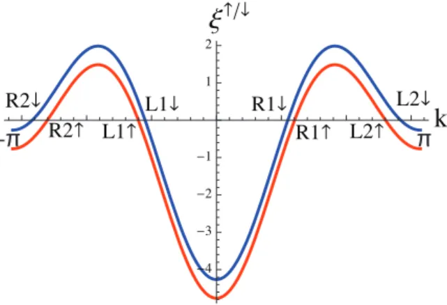
An important question is whether the field can cause changes in the physical state of the system. To this end, we explore possible instabilities of the two-legged SBM state in the Zeeman field.

Figure 4.1: Single-particle spectrum in the presence of the Zeeman field, ξ ↑/↓ (k) =

Transition to Mott insulator: SBM phase

In this case, the scaling dimensions remain larger than 2 and the SBM phase remains stable under the Zeeman field. We see that in the absence of the residual interactions, the SBM remains stable under the Zeeman field.

Figure 4.4: Scaling dimensions ∆[w ↑ 12 ] and ∆[w 12 ↓ ] as a function of h/t 1 for fixed t 2 /t 1 = 1, calculated in the absence of residual spinon interactions

Observables in the SBM in Zeeman field

We can also view (x)∼Sz(x) in the same sense because of the presence of the Zeeman energy. Due to the pinning condition on the θρ+, only the PQ=π+,(n=odd) are non-zero, and we can use the nearest magnon pair operatorP+,(1) as the main representative.

Nearby phases out of the SBM in the field

In the present SBM problem, the main spin-2 observables occur exactly at Q= 0, π, and we give bosonized expressions only for these. Having discussed the observables controlled by the gapless+ part, let us finally mention that Bπ(1) and χπ directly reveal the gapless ϕ−↓ field, cf.

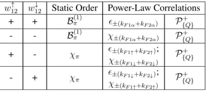
Phases when both w 12 ↑ and w ↓ 12 are relevant

w ↑ 12 > 0, w ↓ 12 > 0
w ↑ 12 < 0, w ↓ 12 < 0
w ↑ 12 > 0, w ↓ 12 < 0
w ↑ 12 < 0, w ↓ 12 > 0

We cannot tell which of the various cases are most likely in particular microscopic models. The power-law correlation exponents also depend on the unknown Luttinger parameter gσ+ in the "σ+" field, and we cannot tell whether spin-2 or spin-0 observables dominate (their scaling dimensions are 1/gσ+oggσ+/4 , respectively).

Table 4.2: Summary of the cases when both w 12 ↑ and w 12 ↓ terms are relevant. For w 12 ↑ w 12 ↓ > 0 we have period-2 VBS order, while for w 12↑ w 12↓ < 0 we have period-2 chirality order

Discussion

Let us apply the weak coupling (RG) renormalization group to study the effects of electronic interactions in the presence of the orbital magnetic field. The stability in the spin sector is then determined by the signs of the λσ bonds.

Figure 5.1: Top: Zigzag strip with uniform flux Φ penetrating each triangular plaquette.

Observables in the Mott-insulating phase in orbital field

After expanding in terms of continuum fields in each case, we find that all cases can be summarized by a single form that requires only the physical coordination but not the sublattice labels: After expanding in terms of continuum fields, we find that both cases can be summarized by a single form that only requires the physical coordinate, .

Spin-gapped phases in orbital field

λ σ 11 < 0, λ σ 22 > 0, λ σ 12 > 0
λ σ 11 > 0, λ σ 22 < 0, λ σ 12 > 0
λ σ 11 , λ σ 22 > 0, λ σ 12 < 0
λ σ 11 , λ σ 22 < 0, λ σ 12 > 0
λ σ 12 < 0 and either λ σ 11 < 0 or λ σ 22 < 0

The instabilities depend on the signs of the λσ11, λσ22 and λσ12 couplings, so there are eight cases. Here, we do not know how to minimize the relevant interactions due to the competition of the pinning terms in V⊥, Eq.

Figure 5.3: Top: Period-4 translational symmetry breaking when λ σ 11 , λ σ 22 > 0, λ σ 12 < 0, drawn in the 1D chain picture

Discussion

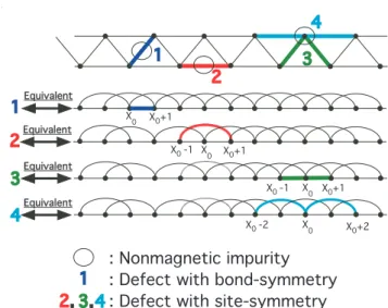
Nonmagnetic defects treated as perturbations

Physically, this leads to the chain being split into two decoupled semi-infinite systems, which we can then study separately. Below we will consider a fixed point of a semi-infinite system and provide physical calculations of the bond textures and the oscillatory sensitivity near the boundary (impurity).

Figure 6.1: The top figure represents the original 2-leg triangular ladder model with ring exchanges, and the thick lines represent the defects due to the impurities

Physical calculations of oscillating susceptibility and bond textures

The pinning value of the fieldθρ− depends on the details such as the amplitudes and phases γ in Eq. Knowing the fixed point theory of the semi-infinite chain, we can briefly discuss other situations of impurities.

Other situations with impurities

Weakly coupled semi-infinite systems
Spin- 1 2 impurity coupled to a semi-infinite system

The situation is more complex than in the previous subsection, because we now have symmetry between the two semi-infinite systems, reminiscent of the 2-channel Kondo problem. When all couplings are marginally irrelevant, the impurity spin and the two semi-infinite systems will decouple at low energies (and the physical calculations of textures in section 6.1.2 are valid in this case).

Conclusions

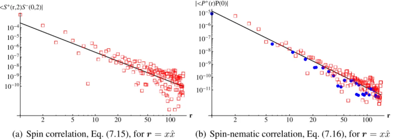
In Section 7.2.2, we present the exact numerical calculations of spin correlations and spin-nematic correlations. In this case, 2m = 4 and therefore two bands are enough to obtain a complete solution of the Majorano problem.

Figure 7.1: Graphical representation of the exactly solvable Kitaev-type model and its so- so-lution in the zero flux sector

Correlation functions

Long wavelength analysis

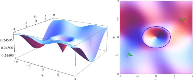
For the long-wavelength description of spin-nematic correlations, we can in principle relate the expression of the spin operator, Eq. The above implies that the spin-nematic correlations contain dominant contributions to the wave vectorsq=0,kF R−kF L,±(kF R+kF L).

Exact numerical calculation

The first and second equations are singular from the inside of the central "ring", and the closed rings sit roughly on a diagonal of B.Z. Theq =±(kF R+kF L)singular lines (small triangles) are quite weak, but. a) Three-dimensional view of the spin structure factor (b) Top view of the spin structure factor.

Figure 7.3: Figures (a) and (b) illustrate power-law behaviors of the spin correlations and spin-nematic correlations

Majorana spin liquid in the Zeeman field

The inner blue ring specifies the line atkF R−kF L; the red closed rings specify the lines at ±2kF; the small green triangles specify the lines on ±(kF R+kF L). still visible, and their locations can be seen more clearly in the top view shown in Figure a) Three-dimensional view of the spin nematic structure factor. First, the field increases to a threshold value, roughly Bz = 0.024, at which the Fermi surface of the f vanishes and there is a discontinuity in the slope of the magnetization curve, shown in the inset in Figure 1.

Figure 7.5: (a) 3D view of the spin-nematic structure factor, D 2 (q), defined in Eq. (7.20).

Discussion

Fixed-point theory of Majorana orbital liquid and observables

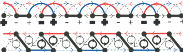
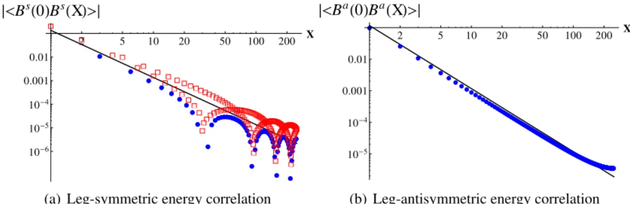
For illustration, we calculate correlations in the exactly solvable model, taking the same parameters as in Fig. We can see the overall X−2 envelope in both figures and also incommensurate oscillations in the symmetric bond-energy correlations, which confirm the theoretical analysis above.

Figure 8.2: Figures (a) and (b) illustrate power law behaviors of the symmetric and anti- anti-symmetric bond energy correlations, with B s/a defined in Eq

Stability of Majorana orbital liquid

Evaluation of expectation value of the string operator in the free fermion ground state leads to a Pfaffian of a matrix formed by the Majorana contractions and can be easily calculated numerically for reasonable sizes [162]. As we discuss in Appendix 8.A, allowing Z2 gauge field fluctuations in the (1+1)D space-time is like allowing half-vortices in the phase field in the bosonized harmonic fluid description and corresponds to allowing termsλ1 / 2cos(θ+kFX+α1/2) in the double harmonic fluid description,.

Figure 8.5: Structure factor corresponding to Fig. 8.4; we also mark the expected locations of the singularities, ±k F .

Gapless SU(2)-invariant Majorana spin liquid (MSL) on the two-leg ladder 155

In the presence of a Zeeman field, the rotational symmetry of the SU(2) spin is broken and only Sz is preserved. We can see that for three identical flavors with incommensurate n¯ , as occurs in SU(2)-invariant MSL, the effects of destructive interference will wash out all vison insertions (including any combinations with non-vison terms).