Statistical and Numerical Methods for Chemical Engineers

(1)

Statistical and Numerical Methods for Chemical Engineers

Part on Statistics

Lukas Meier, ETH Zürich

Lecture Notes of W. Stahel (ETH Zürich) and A. Ruckstuhl (ZHAW)

November 2014

(2)

1 Preliminary Remarks

a Several types of problems lead to statistical models that are highly relevant for chemical engineers:

• A response variable like yield or quality of a product or the duration of a production process may be inﬂuenced by a number of variables – plausible examples are temperature, pressure, humidity, properties of the input material (educts).

– In a ﬁrst step, we need a model for describing the relations. This leads to regression and analysis of variance models. Quite often, simple or multiplelinear regression already give good results.

– Optimization of production processes: If the relations are modelled adequately, it is straightforward to search for those values of the variables that drive the response variable to an optimal value. Methods to eﬃciently ﬁnd these optimum values are discussed under the label of design of ex- periments.

• Chemical processes develop according to clear laws (“law and order of chemical change”, Swinbourne, 1971), which are typically modelled by diﬀerential equations. In these systems there are constants, like the reaction rates, which can be determined from data of suitable experiments. In the simplest cases this leads to linear regression, but usually, the methods of non-linear regression, possibly combined with the numerical solution of diﬀerential equations, are needed. We call this combination system analysis.

• As an efficient surrogate for chemical determination of concentrations of different compounds, indirect determination by spectroscopical measurements are often suitable. Methods that allow for inferring amounts or concentrations of chemical compounds from spectra belong to the field of multivariate statistics.

b In the very limited time available in this course we will present an introduction to these topics. We start with linear regression, a topic you should already be familiar with. The simple linear regression model is used to recall basic statistical notions. The following steps are common for statistical methods:

1. State the scientiﬁc question and characterize the data which are available or will be obtained.

2. Find a suitable probability model that corresponds to the knowledge about the processes leading to the data. Typically, a few unknown constants remain, which we call “parameters” and which we want to learn from the data. The model can (and should) be formulated before the data is available.

3. The ﬁeld of statistics encompasses the methods that bridge the gap between models and data. Regarding parameter values, statistics answers the following questions:

a) Which value is the most plausible one for a parameter? The answer is given by estimation. An estimator is a function that determines a parameter value from the data.

b) Is a given value for the parameter plausible? The decision is made by using

1

(4)

a statisticaltest.

c) Which values are plausible? The answer is given by a set of all plausible values, which is usually an interval, the so calledconﬁdence interval.

4. In many applications the prediction of measurements (observations) that are not yet available is of interest.

c Linear regression was already discussed in “Grundlagen der Mathematik II”. Please have a look at your notes to (again) get familiar with the topic.

You ﬁnd additional material for this part of the course on

http://stat.ethz.ch/˜meier/teaching/cheming

(5)

2 Summary of Linear Regression

2.1 Simple Linear Regression

a Assume we have n observations (xi, Yi), i = 1, . . . , n and we want to model the relationship between a response variable Y and a predictor variable x.

Thesimple linear regression modelis

Y_i=α+βx_i+E_i, i= 1, . . . , n.

The x_i’s are ﬁxed numbers while the E_i’s are random, called “random deviations” or

“random errors”. Usual assumptions are

E_i∼N(0,σ²), Ei independent.

The parameters of the simple linear regression model are the coeﬃcients α,β and the standard deviation σ of the random error.

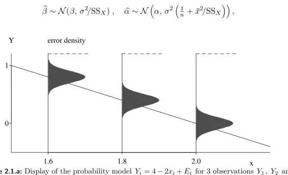
Figure 2.1.a illustrates the model.

b Estimation of the coeﬃcientsfollows the principle of least squaresand yields β�= ^�ⁿⁱ⁼¹(Y_i−Y)(x_i−x)

�n

i=1(xi−x)² , α_�=Y −β^�x .

The estimates β^� and α� ﬂuctuate around the true (but unknown) parameters. More precisely, the estimates are normally distributed,

β�∼N(β,σ²/SSX), α_�∼N^�α,σ²^�_n¹ +x²/SSX

��,

1.6 1.8 2.0

0 1

x

Y error density

Figure 2.1.a:Display of the probability model Yi= 4−2xi+Ei for 3 observations Y1, Y2 and Y3 corresponding to the x values x1= 1.6, x2= 1.8 and x3= 2.

3

(6)

4 2 Summary of Linear Regression

where SSX =^�ⁿ_i=1(xi−x)².

c The deviations of the observed Y_i from the ﬁtted values y�_i = α�+βx^� _i are called residuals Ri =Yi−y�i and are “estimators” of the random errors Ei.

They lead to an estimate of the standard deviation σ of the error,

�

σ² = 1 n−2

�n i=1

R²_i .

d Testof the null hypothesis β =β₀: The test statistic T = β^�−β₀

se(β)^� , se(β^�) =^�σ�²/SSX

has a t-distribution with n−2 degrees of freedom under the null-hypothesis.

This leads to the conﬁdence interval of

β�±q_0.975^tⁿ⁻² se(β).^�

e The “conﬁdence band” for the value of the regression function connects the end points of the conﬁdence intervals for E(Y |x) =α+βx.

Aprediction intervalshall include a (yet unknown) value Y₀ of the response variable for a given x₀ – with a given “statistical certainty” (usually 95%). Connecting the end points for all possible x₀ produces the “prediction band”.

2.2 Multiple Linear Regression

a Compared to the simple linear regression model we now have several predictors x⁽¹⁾, . . . , x^(m).

The multiple linear regression modelis

Y_i = β₀+β₁x⁽¹⁾_i +β₂x⁽²⁾_i +...+β_mx^(m)_i +E_i E_i ∼ N(0,σ²), Ei independent.

In matrix notation:

Y = Xβ+E , E∼Nn(0,σ²I),

where the response vector Y ∈ Rⁿ, the design matrix X ∈ Rⁿ^×^p, the parameter vector β∈R^p and the error vector E ∈Rⁿ for p=m+ 1 (number of parameters).

Y =





 Y₁ Y₂ ...

Yn





, X =







1 x⁽¹⁾₁ x⁽²⁾₁ . . . x^(m)₁ 1 x⁽¹⁾₂ x⁽²⁾₂ . . . x^(m)₂ ... ... ... ... ...

1 x⁽¹⁾n x⁽²⁾n . . . x^(m)n





 , β=





 β₀ β₁ ...

βm





, E=





 E₁ E₂ ...

En





. Diﬀerent rows of the design matrix X are diﬀerent observations. The variables (predictors) can be found in the corresponding columns.

(7)

2.2 Multiple Linear Regression 5

b Estimation is again based on least squares, leading to β�= (X^TX)⁻¹X^TY , i.e. we have a closed form solution.

From the distribution of the estimated coeﬃcients, β�j ∼N

�

βj,σ²^�(X^TX)⁻¹^�

jj

�

t-tests and conﬁdence intervals for individual coeﬃcients can be derived as in the linear regression model. The test statistic

T = β^�_j−β_j,0

se(β^�j) , se(β^�_j) =^�σ�²^�(X^TX)⁻¹^�

jj

follows a t-distribution with n−(m+ 1) parameters under the null-hypothesis H₀ : β_j =β_j,0.

The standard deviation σ is estimated by

�

σ²= 1 n−p

�n i=1

R²_i.

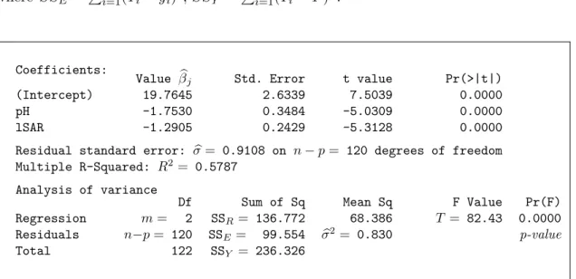
c Table 2.2.c shows a typical computer output, annotated with the corresponding mathematical symbols.

Themultiple correlation R is the correlation between the ﬁtted values y�_i and the observed values Yi. Its square measures the portion of the variance of the Yi’s that is

“explained by the regression”, and is therefore calledcoeﬃcient of determination:

R² = 1−SSE/SSY, where SS_E =^�ⁿ_i=1(Y_i−y�_i)², SS_Y =^�ⁿ_i=1(Y_i−Y)².

Coefficients: Value β�j Std. Error t value Pr(>|t|)

(Intercept) 19.7645 2.6339 7.5039 0.0000

pH -1.7530 0.3484 -5.0309 0.0000

lSAR -1.2905 0.2429 -5.3128 0.0000

Residual standard error: σ�= 0.9108 on n−p= 120 degrees of freedom Multiple R-Squared: R²= 0.5787

Analysis of variance

Df Sum of Sq Mean Sq F Value Pr(F) Regression m= 2 SSR= 136.772 68.386 T = 82.43 0.0000 Residuals n−p= 120 SSE= 99.554 σ�²= 0.830 p-value

Total 122 SSY = 236.326

Table 2.2.c:Computer output for a regression example, annotated with mathematical symbols.

d

(8)

6 2 Summary of Linear Regression The model is called linear because it is linear in the parameters β₀, . . . ,βm. It could well be that some predictors are non-linear functions of other predictors (e.g., x⁽²⁾ = (x⁽¹⁾)²). It is still a linear model as long as the parameters appear in linear form!

e In general, it is not appropriate to replace a multiple regression model by many simple regressions (on single predictor variables).

In a multiple linear regression model, the coefficients describe howY is changing when varying the corresponding predictor and keeping the other predictor variables constant. I.e., it is the effect of the predictor on the responseafter having subtracted the effect of all other predictors on Y. Hence we need to have all predictors in the model at the same time in order to estimate this effect.

f Many applications The model of multiple linear regression model is suitable for describing many diﬀerent situations:

• Transformationsof the predictors (and the response variable) may turn origi- nally non-linear relations into linear ones.

• A comparison of two groups is obtained by using a binary predictor variable.

Several groups need a “block of dummy variables”. Thus, nominal (or cate- gorical) explanatory variablescan be used in the model and can be combined with continuous variables.

• The idea of diﬀerent linear relations of the response with some predictors in diﬀerent groups of data can be included into a single model. More generally,in- teractionsbetween explanatory variables can be incorporated by suitable terms in the model.

• Polynomial regression is a special case of multiple linear (!) regression (see example above).

g TheF-Test for comparison of modelsallows for testing whether several coeﬃcients are zero. This is needed for testing whether a categorical variable has an inﬂuence on the response.

2.3 Residual Analysis

a The assumptions about the errors of the regression model can be split into

(a) their expected values are zero: E(Ei) = 0 (or: the regression function is correct),

(b) they have constant variance, Var(Ei) =σ², (c) they arenormally distributed,

(d) they areindependent of each other.

These assumptions should be checked for

• deriving a better model based on deviations from it,

• justifying tests and conﬁdence intervals.

Deviations are detected by inspecting graphical displays. Tests for assumptions play a less important role.

(9)

2.3 Residual Analysis 7

b Fitting a regression model without examining the residuals is a risky exer- cise!

c The following displays are useful:

(a) Non-linearities: Scatterplot of (unstandardized) residuals againstﬁtted values (Tukey-Anscombe plot)and against the (original)explanatory variables.

Interactions: Pseudo-threedimensional diagram of the (unstandardized) residuals against pairs of explanatory variables.

(b) Equal scatter: Scatterplot of (standardized) absolute residuals against ﬁtted values (Tukey-Anscombe plot) and against (original) explanatory vari- ables. Usually no special displays are given, but scatter is examined in the plots for (a).

(c) Normal distribution: QQ-plot (or histogram) of (standardized) residuals.

(d) Independence: (unstandardized) residuals against time or location.

(e) Inﬂuential observations for the ﬁt: Scatterplot of (standardized) residuals againstleverage.

Inﬂuential observations for individual coeﬃcients: added-variable plot.

(f) Collinearities: Scatterplot matrix of explanatory variables and numerical output (of R²_j or VIFj or “tolerance”).

d Remedies:

• Transformation (monotone non-linear) of the response: if the distribution of the residuals is skewed, for non-linearities (if suitable) or unequal variances.

• Transformation (non-linear) of explanatory variables: when seeing non- linearities, high leverages (can come from skewed distribution of explanatory variables) and interactions (may disappear when variables are transformed).

• Additional terms: to model non-linearities and interactions.

• Linear transformations of several explanatory variables: to avoid collinearities.

• Weighted regression: if variances are unequal.

• Checking the correctness of observations: for all outliers in any display.

• Rejection of outliers: if robust methods are not available (see below).

More advanced methods:

• Generalized least squares: to account for correlated random errors.

• Non-linear regression: if non-linearities are observed and transformations of variables do not help or contradict a physically justiﬁed model.

• Robust regression: should always be used, suitable in the presence of outliers and/or long-tailed distributions.

Note that correlations among errors lead to wrong test results and conﬁdence intervals which are most often too short.

(10)

3 Nonlinear Regression

3.1 Introduction

a The Regression Model Regression studies the relationship between a variable of interest Y and one or moreexplanatory or predictor variables x^(j). The general model is

Y_i =h(x⁽¹⁾_i , x⁽²⁾_i , . . . , x^(m)_i ;θ₁,θ₂, . . . ,θ_p) +E_i.

Here, h is an appropriate function that depends on the predictor variables and parameters, that we want to summarize with vectors x = [x⁽¹⁾_i , x⁽²⁾_i , . . . , x^(m)_i ]^T and θ = [θ1,θ₂, . . . ,θ_p]^T. We assume that the errors are all normally distributed and independent, i.e.

E_i∼N^�0,σ²^�, independent.

b The Linear Regression Model In (multiple) linear regression, we considered functions h that are linear in the parameters θj,

h(x⁽¹⁾_i , x⁽²⁾_i , . . . , x^(m)_i ;θ₁,θ₂, . . . ,θ_p) =θ₁x_�⁽¹⁾_i +θ₂x_�⁽²⁾_i +. . .+θ_px_�^(p)_i ,

where the x�^(j) can be arbitrary functions of the original explanatory variables x^(j). There, the parameters were usually denoted by β_j instead of θ_j.

c The Nonlinear Regression Model In nonlinear regression, we use functions h that are not linear in the parameters. Often, such a function is derived from theory. In principle, there are unlimited possibilities for describing the deterministic part of the model. As we will see, this ﬂexibility often means a greater eﬀort to make statistical statements.

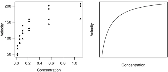
Example d Puromycin The speed of an enzymatic reaction depends on the concentration of a substrate. As outlined in Bates and Watts (1988), an experiment was performed to examine how a treatment of the enzyme with an additional substance called Puromycin inﬂuences the reaction speed. The initial speed of the reaction is chosen as the response variable, which is measured via radioactivity (the unit of the response variable is count/min²; the number of registrations on a Geiger counter per time period measures the quantity of the substance, and the reaction speed is proportional to the change per time unit).

The relationship of the variable of interest with the substrate concentrationx (in ppm) is described by the Michaelis-Menten function

h(x;θ) = θ₁x θ₂+x .

An inﬁnitely large substrate concentration (x → ∞) leads to the “asymptotic” speed θ₁. It was hypothesized that this parameter is inﬂuenced by the addition of Puromycin.

The experiment is therefore carried out once with the enzyme treated with Puromycin

8

(11)

3.1 Introduction 9

0.0 0.2 0.4 0.6 0.8 1.0 50

100 150 200

Concentration

Velocity

Concentration

Velocity

Figure 3.1.d:Puromycin. (a) Data (• treated enzyme; � untreated enzyme) and (b) typical shape of the regression function.

1 2 3 4 5 6 7

8 10 12 14 16 18 20

Days

Oxygen Demand

Days

Oxygen Demand

Figure 3.1.e:Biochemical Oxygen Demand. (a) Data and (b) typical shape of the regression function.

and once with the untreated enzyme. Figure 3.1.d shows the data and the shape of the regression function. In this section only the data of the treated enzyme is used.

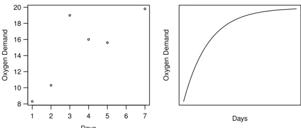
Example e Biochemical Oxygen DemandTo determine the biochemical oxygen demand, stream water samples were enriched with soluble organic matter, with inorganic nutrients and with dissolved oxygen, and subdivided into bottles (Marske, 1967, see Bates and Watts, 1988). Each bottle was inoculated with a mixed culture of microorganisms, sealed and put in a climate chamber with constant temperature. The bottles were periodically opened and their dissolved oxygen concentration was analyzed, from which the biochemical oxygen demand [mg/l] was calculated. The model used to connect the cumulative biochemical oxygen demand Y with the incubation time x is based on exponential decay:

h(x;θ) =θ₁^�1−e⁻^θ²^x^�.

Figure 3.1.e shows the data and the shape of the regression function.

(12)

10 3 Nonlinear Regression

2 4 6 8 10 12

160 161 162 163

x (=pH)

y (= chem. shift)

(a)

x

y

(b)

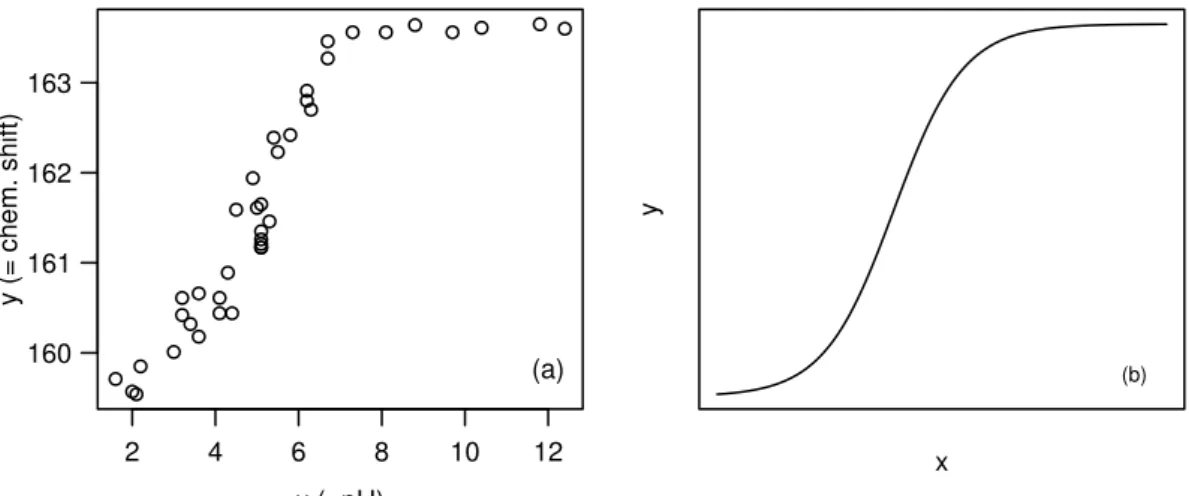
Figure 3.1.f:Membrane Separation Technology. (a) Data and (b) a typical shape of the regression function.

Example f Membrane Separation TechnologySee Rapold-Nydegger (1994). The ratio of proto- nated to deprotonated carboxyl groups in the pores of cellulose membranes depends on the pH-value x of the outer solution. The protonation of the carboxyl carbon atoms can be captured with ¹³C-NMR. We assume that the relationship can be written with the extended “Henderson-Hasselbach Equation” for polyelectrolytes

log₁₀^�θ₁−y y−θ₂

� =θ₃+θ₄x ,

where the unknown parameters are θ₁,θ₂ and θ₃>0 and θ₄ <0. Solving for y leads to the model

Y_i =h(xi;θ) +E_i = θ₁+θ₂10^θ³^+θ⁴^xⁱ 1 + 10^θ³^+θ⁴^xⁱ +E_i .

The regression function h(xi,θ) for a reasonably chosen θ is shown in Figure 3.1.f next to the data.

g A Few Further Examples of Nonlinear Regression Functions

• Hill model (enzyme kinetics): h(xi,θ) =θ₁x^θ_i³/(θ2+x^θ_i³)

For θ₃ = 1 this is also known as the Michaelis-Menten model (3.1.d).

• Mitscherlich function (growth analysis): h(xi,θ) =θ₁+θ₂exp(θ3x_i).

• From kinetics (chemistry) we get the function

h(x⁽¹⁾_i , x⁽²⁾_i ;θ) = exp(−θ₁x⁽¹⁾_i exp(−θ₂/x⁽²⁾_i )).

• Cobbs-Douglas production function

h^�x⁽¹⁾_i , x⁽²⁾_i ;θ^� =θ₁ ^�x⁽¹⁾_i ^�^θ² ^�x⁽²⁾_i ^�^θ³.

Since useful regression functions are often derived from the theoretical background of the application of interest, a general overview of nonlinear regression functions is of very limited beneﬁt. A compilation of functions from publications can be found in Appendix 7 of Bates and Watts (1988).

h Linearizable Regression Functions Some nonlinear regression functions can be lin- earized by transformations of the response variable and the explanatory variables.

(13)

3.1 Introduction 11

For example, a power function

h(x;θ) =θ₁x^θ²

can be transformed to a linear (in the parameters!) function ln(h(x;θ)) = ln(θ1) +θ₂ln(x) =β₀+β₁x ,_�

where β₀ = ln(θ₁), β₁ = θ₂ and x� = ln(x). We call the regression function h linearizable, if we can transform it into a function that is linear in the (unknown) parameters by (monotone) transformations of the arguments and the response.

Here are some more linearizable functions (see also Daniel and Wood, 1980):

h(x;θ) = 1/(θ1+θ2exp(−x)) ←→ 1/h(x;θ) =θ1+θ2exp(−x) h(x;θ) =θ1x/(θ2+x) ←→ 1/h(x;θ) = 1/θ1+θ2/θ11

x

h(x;θ) =θ1x^θ² ←→ ln(h(x;θ)) = ln(θ1) +θ2ln(x) h(x;θ) =θ1exp(θ2g(x)) ←→ ln(h(x;θ)) = ln(θ1) +θ2g(x)

h(x;θ) = exp(−θ1x⁽¹⁾exp(−θ2/x⁽²⁾)) ←→ ln(ln(h(x;θ))) = ln(−θ1) + ln(x⁽¹⁾)−θ2/x⁽²⁾ h(x;θ) =θ1 �

x⁽¹⁾�θ2 � x⁽²⁾�θ3

←→ ln(h(x;θ)) = ln(θ1) +θ2 ln(x⁽¹⁾) +θ3 ln(x⁽²⁾).

The last one is the Cobbs-Douglas Model from 3.1.g.

i A linear regression with the linearized regression function of the example above is based on the model

ln(Yi) =β₀+β₁x_�_i+E_i,

where the random errors E_i all have the same normal distribution. We transform this model back and get

Yi =θ₁·x^θ² ·E^�i,

with E^�i = exp(Ei). The errors E^�i, i= 1, . . . , n, now have a multiplicative eﬀect and are log-normally distributed! The assumptions about the random deviations are thus now drastically diﬀerent than for a model that is based directly on h,

Y_i =θ₁·x^θ² +E_i^∗,

with random deviations E_i^∗ that, as usual, contribute additively and have a speciﬁc normal distribution.

A linearization of the regression function is therefore advisable only if the assumptions about the random errors can be better satisﬁed – in our example, if the errors actually act multiplicatively rather than additively and are log-normally rather than normally distributed. These assumptions must be checked with residual analysis.

j *Note: For linear regression it can be shown that the variance can be stabilized with certain transformations (e.g. log(·),√

·). If this is not possible, in certain circumstances one can also perform a weighted linear regression. The process is analogous in nonlinear regression.

(14)

12 3 Nonlinear Regression k We have almost exclusively seen regression functions that only depend on one predictor variable x. This was primarily because it was possible to graphically illustrate the model. The following theory also works well for regression functions h(x;θ) that depend on several predictor variables x= [x⁽¹⁾, x⁽²⁾, . . . , x^(m)].

3.2 Parameter Estimation

a The Principle of Least SquaresTo get estimates for the parameters θ= [θ1, θ₂, . . ., θp]^T, one applies – like in linear regression – the principle of least squares. The sum of the squared deviations

S(θ) :=^�ⁿ

i=1

(yi−ηi(θ))² where ηi(θ) :=h(xi;θ)

should be minimized. The notation that replaces h(xi;θ) with ηi(θ) is reasonable because [xi, y_i] is given by the data and only the parametersθremain to be determined.

Unfortunately, the minimum of S(θ) and hence the estimator have no explicit solution (in contrast to the linear regression case). Iterative numeric procedures are therefore needed. We will sketch the basic ideas of the most common algorithm. It is also the basis for the easiest way to derive tests and conﬁdence intervals.

b Geometrical Illustration The observed values Y = [Y1, Y₂, . . . , Yn]^T deﬁne a point in n-dimensional space. The same holds true for the “model values” η(θ) = [η₁(θ),η₂(θ), . . . ,η_n(θ)]^T for a given θ.

Please take note: In multivariate statistics where an observation consists of mvariables x^(j), j= 1,2, . . . , m, it’s common to illustrate the observations in the m-dimensional space. Here, we consider the Y- and η-values of all n observations as points in the n-dimensional space.

Unfortunately, geometrical interpretation stops with three dimensions (and thus with three observations). Nevertheless, let us have a look at such a situation,ﬁrst for simple linear regression.

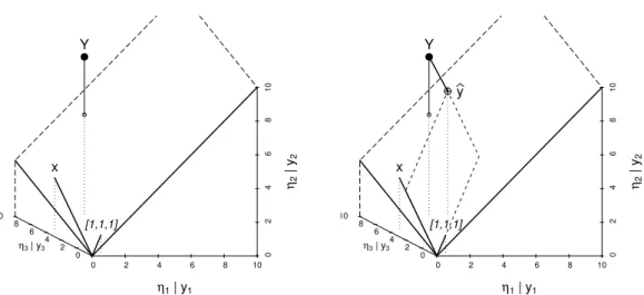
c As stated above, the observed values Y = [Y1, Y₂, Y₃]^T determine a point in three- dimensional space. For given parameters β₀ = 5 andβ₁ = 1 we can calculate the model values η_i^�β^�=β₀+β₁x_i and represent the corresponding vector η^�β^�=β₀1 +β₁x as a point. We now ask: Where are all the points that can be achieved by varying the parameters? These are the possible linear combinations of the two vectors 1 and x: they form a plane “spanned by 1 and x”. By estimating the parameters according to the principle of least squares, the squared distance between Y and η^�β^� is minimized. This means that we are looking for the point on the plane that is closest to Y . This is also called theprojection of Y onto the plane. The parameter values that correspond to this point η� are therefore the estimated parameter values β�= [β^�₀,β^�₁]^T. An illustration can be found in Figure 3.2.c.

d Now we want to ﬁt a nonlinear function, e.g. h(x;θ) =θ₁exp(1−θ₂x), to the same three observations. We can again ask ourselves: Where are all the points η(θ) that can be achieved by varying the parameters θ₁ and θ₂? They lie on a two-dimensional curvedsurface (called themodel surfacein the following) in three-dimensional space.

The estimation problem again consists ofﬁnding the point η�on the model surface that is closest to Y. The parameter values that correspond to this point η� are then the

(15)

3.2 Parameter Estimation 13

0 2 4 6 8 10 0 2 4 6 810 2 0

6 4 10 8

η1 | y1

η2 | y2

η3 | y3

Y

[1,1,1]

x

0 2 4 6 8 10 0 2 4 6 810 2 0

6 4 10 8

η1 | y1

η2 | y2

η3 | y3

Y

[1,1,1]

x

y

Figure 3.2.c:Illustration of simple linear regression. Values of η�

β� = β0+β1x for varying parameters [β0,β1] lead to a plane in three-dimensional space. The right plot also shows the point on the surface that is closest to Y = [Y1, Y₂, Y₃]. It is theﬁtted valuey�and determines the estimated parameters β�.

estimated parameter values θ^�= [θ^�₁,θ^�₂]^T. Figure Figure 3.2.d illustrates the nonlinear case.

5 6 7 8 9 10 11

101214161820

19 18 21 20 22

η1 | y1

η2 | y2

η₃ | y₃

− Y

Figure 3.2.d:Geometrical illustration of nonlinear regression. The values of η(θ) =h(x;θ₁,θ₂) for varying parameters [θ1,θ₂] lead to a two-dimensional “model surface” in three-dimensional space. The lines on the model surface correspond to constant η₁ and η₃, respectively.

(16)

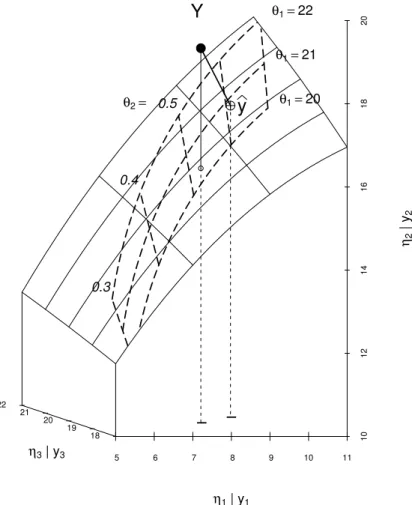
14 3 Nonlinear Regression e Biochemical Oxygen Demand (cont’d) The situation for our Biochemical Oxygen Demand example can be found in Figure 3.2.e. Basically, we can read the estimated parameters directly oﬀthe graph here: θ^�₁ is a bit less than 21 and θ^�₂ is a bit larger than 0.6. In fact the (exact) solution is θ^�= [20.82,0.6103] (note that these are the parameter estimates for the reduced data set only consisting of three observations).

5 6 7 8 9 10 11

101214161820

19 18 21 20 22

η1 | y1

η2 | y2

η₃ | y₃

− Y

θ1=20 θ1=21 θ₁=22

0.3 0.4

θ₂= 0.5

− y

Figure 3.2.e:Biochemical Oxygen Demand: Geometrical illustration of nonlinear regression.

In addition, we can see here the lines of constant θ1 and θ2, respectively. The vector of the estimated model values y�=h�

x;θ��

is the point on the model surface that is closest to Y. f Approach for the Minimization Problem The main idea of the usual algorithm for

minimizing the sum of squares (see 3.2.a) is as follows: If a preliminary best value θ^(�) exists, we approximate the model surface with the plane that touches the surface at the point η^�θ^(�)^�=h^�x;θ^(�)^� (the so called tangent plane). Now, we are looking for the point on that plane that lies closest to Y . This is the same as estimation in a linear regression problem. This new point lies on the plane, but not on the surface that corresponds to the nonlinear problem. However, it determines a parameter vector θ^(�+1) that we use as starting value for the next iteration.

g Linear Approximation To determine the tangent plane we need the partial derivatives A^(j)_i (θ) := ∂ηi(θ)

∂θ_j ,

that can be summarized by an n×p matrix A. The approximation of the model

(17)

3.2 Parameter Estimation 15

surface η(θ) by the tangent plane at a parameter value θ^∗ is

η_i(θ)≈η_i(θ^∗) +A⁽¹⁾_i (θ^∗) (θ1−θ₁^∗) +...+A^(p)_i (θ^∗) (θp−θ^∗_p) or, in matrix notation,

η(θ)≈η(θ^∗) +A(θ^∗) (θ−θ^∗). If we now add a random error, we get a linear regression model

Y� = A(θ^∗)β+E

with “preliminary residuals” Y^�_i=Y_i−η_i(θ^∗) as response variable, the columns of A as predictors and the coeﬃcients β_j =θ_j−θ_j^∗ (a model without intercept β₀).

h Gauss-Newton Algorithm The Gauss-Newton algorithm starts with an initial value θ⁽⁰⁾ for θ, solving the just introduced linear regression problem for θ^∗ =θ⁽⁰⁾ toﬁnd a correction β and hence an improved value θ⁽¹⁾ =θ⁽⁰⁾+β. Again, the approximated model is calculated, and thus the “preliminary residuals” Y −η^�θ⁽¹⁾^� and the partial derivatives A^�θ⁽¹⁾^� are determined, leading to θ₂. This iteration step is continued until the the correction β is small enough.

It can not be guaranteed that this procedure actuallyﬁnds the minimum of the sum of squares. The better the p-dimensional model surface can be locally approximated by a p-dimensional plane at the minimum θ^�= (θ^�₁, . . . ,θ^�_p)^T and the closer the initial value θ⁽⁰⁾ is to the solution, the higher are the chances of ﬁnding the optimal value.

*Algorithms usually determine the derivative matrix A numerically. In more complex problems the numerical approximation can be insuﬃcient and cause convergence problems. For such situations it is an advantage if explicit expressions for the partial derivatives can be used to determine the derivative matrix more reliably (see also Chapter 3.6).

i Initial Values An iterative procedure always requires an initial value. Good initial values help to ﬁnd a solution more quickly and more reliably. Some possibilities to arrive at good initial values are now being presented.

j Initial Value from Prior Knowledge As already noted in the introduction, nonlinear models are often based on theoretical considerations of the corresponding application area. Already existingprior knowledgefrom similar experiments can be used to get an initial value. To ensure the quality of the chosen initial value, it is advisable to graphically represent the regression function h(x;θ) for various possible initial values θ=θ⁰ together with the data (e.g., as in Figure 3.2.k, right).

k Initial Values via Linearizable Regression Functions Often – because of the distribution of the error term – one is forced to use a nonlinear regression function even though it would be linearizable. However, the linearized model can be used to get initial values.

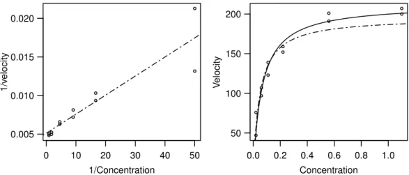
In the Puromycin example the regression function is linearizable: The reciprocal values of the two variables fulﬁll

� y= 1

y ≈ 1

h(x;θ) = 1 θ₁ +θ₂

θ₁ 1

x =β₀+β₁x ._�

The least squares solution for this modiﬁed problem isβ^�= [β^�₀,β^�₁]^T = (0.00511,0.000247)^T (Figure 3.2.k, left). This leads to the initial values

θ⁽⁰⁾₁ = 1/β^�₀ = 196, θ⁽⁰⁾₂ =β^�₁/β^�₀= 0.048.

(18)

16 3 Nonlinear Regression

0 10 20 30 40 50

0.005 0.010 0.015 0.020

1/Concentration

1/velocity

0.0 0.2 0.4 0.6 0.8 1.0 50

100 150 200

Concentration

Velocity

Figure 3.2.k:Puromycin. Left: Regression function in the linearized problem. Right: Regres- sion functionh(x;θ) for the initial valuesθ=θ⁽⁰⁾ ( ) and for the least squares estimation θ=θ�(——–).

l Initial Values via Geometric Interpretation of the Parameter It is often helpful to consider the geometrical features of the regression function.

In the Puromycin Example we can derive an initial value in another way: θ₁ is the response value forx=∞. Since the regression function is monotonically increasing, we can use the maximal yi-value or a visually determined “asymptotic value” θ₁⁽⁰⁾= 207 as initial value for θ₁. The parameter θ₂ is the x-value, such that y reaches half of the asymptotic value θ₁. This leads to θ⁽⁰⁾₂ = 0.06.

The initial values thus result from a geometrical interpretation of the parameters and a rough estimate can be determined by “ﬁtting by eye”.

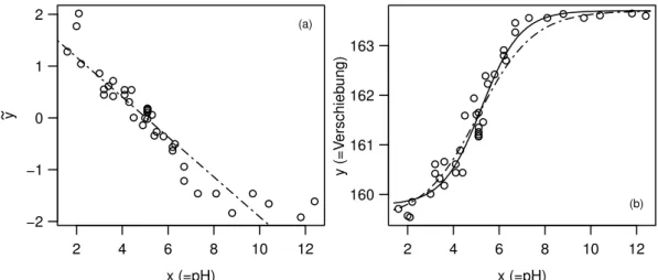
Example m Membrane Separation Technology (cont’d)In the Membrane Separation Technology example we let x→ ∞, so h(x;θ) → θ₁ (since θ₄ <0); for x→ −∞, h(x;θ) → θ₂. From Figure 3.1.f (a) we see that θ₁ ≈163.7 and θ₂ ≈159.5. Once we know θ₁ and θ₂, we can linearize the regression function by

�

y:= log₁₀

�θ⁽⁰⁾₁ −y y−θ₂⁽⁰⁾

�

=θ₃+θ₄x .

This is called aconditional linearizablefunction. The linear regression model leads to the initial value θ⁽⁰⁾₃ = 1.83 and θ₄⁽⁰⁾=−0.36.

With this initial value the algorithm converges to the solution θ^�₁ = 163.7, θ^�₂ = 159.8, θ�₃ = 2.675 and θ^�₄ =−0.512. The functions h(·;θ⁽⁰⁾) and h(·;θ) are shown in Figure^� 3.2.m (b).

*The property of conditional linearity of a function can also be useful to develop an algorithm speciﬁcally suited for this situation (see e.g. Bates and Watts, 1988).

3.3 Approximate Tests and Conﬁdence Intervals

a The estimator θ^� is the value of θ that optimally fits the data. We now ask which parameter values θ are compatible with the observations. The confidence region is the set of all these values. For an individual parameter θ_j the confidence region is a confidence interval.

(19)

3.3 Approximate Tests and Conﬁdence Intervals 17

2 4 6 8 10 12

−2

−1 0 1 2

x (=pH)

y

(a)

2 4 6 8 10 12

160 161 162 163

x (=pH)

y (=Verschiebung)

(b)

Figure 3.2.m:Membrane Separation Technology. (a) Regression line that is used for deter- mining the initial values for θ3 and θ4. (b) Regression function h(x;θ) for the initial value θ=θ⁽⁰⁾ ( ) and for the least squares estimator θ=θ�(——–).

The following results are based on the fact that the estimator θ^�is asymptotically (multivariate) normally distributed. For an individual parameter that leads to a “Z-Test”

and the corresponding conﬁdence interval; for multiple parameters the corresponding Chi-Square test is used and leads to elliptical conﬁdence regions.

b Theasymptotic propertiesof the estimator can be derived from the linear approximation. The problem of nonlinear regression is indeed approximately equal to the linear regression problem mentioned in 3.2.g

Y� = A(θ^∗)β+E ,

if the parameter vector θ^∗ that is used for the linearization is close to the solution. If the estimation procedure has converged (i.e.θ^∗=θ), then^� β = 0 (otherwise this would not be the solution). The standard error of the coeﬃcients β^� – or more generally the covariance matrix of β^� – then approximate the corresponding values of θ.^�

c Asymptotic Distribution of the Least Squares Estimator It follows that the least squares estimator θ^� is asymptotically normally distributed

θ�^as.∼ N(θ,V (θ)),

with asymptotic covariance matrix V (θ) = σ²(A(θ)^T A(θ))⁻¹, where A(θ) is the n×p matrix of partial derivatives (see 3.2.g).

To explicitly determine the covariance matrixV(θ), A(θ) is calculated using θ^�instead of the unknown θ. For the error variance σ² we plug-in the usual estimator

V�(θ) =σ�²

�

A^�θ^�^�^T A^�θ^�^��

−1

where

σ�²= S(θ)^�

n−p = 1 n−p

�n i=1

�y_i−η_i^�θ^�^{� �}².

Hence, the distribution of the estimated parameters is approximately determined and we can (like in linear regression) derive standard errors and conﬁdence intervals, or conﬁdence ellipses (or ellipsoids) if multiple variables are considered jointly.