An important application of the closed topological string theory is the Ooguri, Strominger and Vafa (OSV) conjectures. In the first part of this thesis, we investigate a holomorphic anomaly equation for the open topological string amplitudes.
Topological String Theory
- Introduction
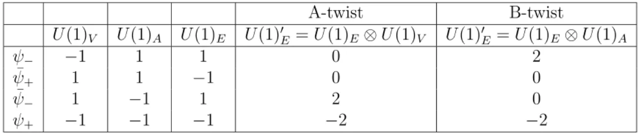
- N = (2, 2) supersymmetry
- Topological sigma model
- U (1) R anomaly
- Closed topological string theory
- Bosonic string theory
- Closed topological string amplitudes
- Relation between closed topological strings and physi- cal stringscal strings
The twisted (2,2) sigma model is topological because the variation of the action with respect to the world sheet metric is Q-exact. Therefore, the anomaly is the same as for the topological sigma model on the Calabi-Yau 3-fold (2.22).
The Open Holomorphic Anomaly Equation
Introduction
In [19] it was shown that D-branes in the A-model are associated with Lagrangian 3-cycles and that their disk one-point functions depend on B-model moduli. Conversely, D-branes in the B-model are associated with holomorphic even cycles, and their disk one-point functions depend on A-model modules.
The open topological string theory
- Boundary condition
- Some aspects of the moduli spaces of Riemann surfaces
- Open holomorphic anomaly equation
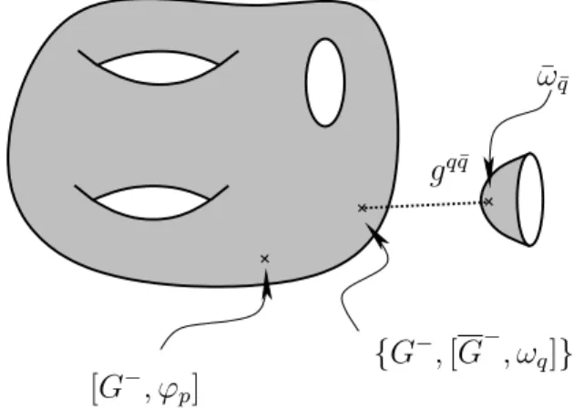
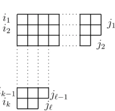
The limit of the moduli space of Riemann surfaces corresponds to various degenerations of the surface (marked points are ignored). Note that in the presence of orientifolds, Cp¯ is the sum of the disc and crosscap one-point functions [20].
New anomalies in topological string theory
- Physical meaning of the new anomalies
- Anomalous worldsheet degenerations
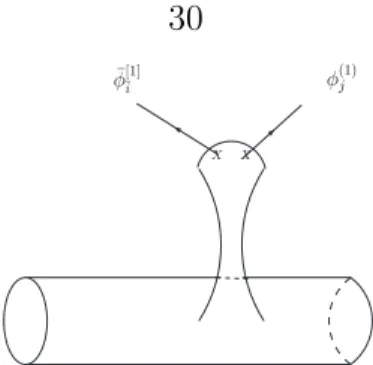
By moving the contour of the supercurrent G++G+ around the Riemann surface, we pick up contributions from the commutation relations. The residual modulus of the created long, thin tube is represented by an integrated (G−−G−) insertion, folded with Beltrami differential. The degeneration produces a thin strip, with each end surrounded by a G- or G- folded with a Beltrami differential, associated with the position of the strip's attachment to the border.
The final interesting case is that of a boundary shrinking or similarly moving far from the rest of the Riemann surface (Figure 3.6). That such a degeneracy is part of the limit of the moduli space can be seen by doubling the Riemann surface Σg,h to form the closed surface Σ′2g+h−1,0, as described in Section 3.2.2. The boundary degeneracy is thus equivalent to a boundary at the end of a long tube, with the Beltrami differences associated with the two remaining moduli localized at the attachment point of the tube with the rest of the Riemann surface.
Small number of moduli
- Cylinder Σ 0 , 2
- Some discussion
If the disk one-point function does not vanish, we get an incorrect modulo-dependent term. When the disc one-point functions vanish, we get the holomorphic anomaly equation for a cylinder. We can repeat the same discussion and find that the only contribution comes from the disk one-point functions, and therefore the vanishing of the disk one-point function makes them all zero.
At the same time, these sinks cancel the one-point features of the disk, and so the appearance of the new anomalies is correlated with an invalid spacetime construction. It is well known that open topological string theory on this space is the U(N) Chern-Simons theory, which is topological and should be independent of the S3 radius. The limit states of the two stacks are combined to give Cp¯= 0 and the new anomalies are not shown.
Feynman rules to solve the holomorphic anomaly equationequation
Now take the limit where the second 3-cycle moves infinitely far from the underlying S3 to recover the local anomaly-free Calabi-Yau construction. The point is that in non-compact Calabi-Yau polyhedra, new anomalies can be removed by a suitable choice of boundary conditions at infinity.
![Figure 3.17: The propagators for Feynman diagrams of topological string amplitudes The low-genus and boundary cases, F (2,0) , F (3,0) , F (1,1) , and F (0,3) , were studied in [1] and [7]](https://thumb-ap.123doks.com/thumbv2/123dok/11430417.0/43.918.163.815.148.434/figure-propagators-feynman-diagrams-topological-amplitudes-boundary-studied.webp)
The Relation between the Open and Closed Topological String
Generating function
The ingredients Fi(g,h)1,..,in are topological string amplitudes with worldsheet genusg, h-bounds and nine insertions of marginal operators with closed strings, indexed byi1, · · · , in; also C¯jki =C¯i¯j¯ke2KGj¯jGkk¯, where C¯i¯j¯k is the Yukawa coupling, indices are increased and decreased using the Zamolodchikov metric Gi¯j = ∂i∂¯ jK, and ∆ ¯ji = eKGj¯k∆¯i¯k, where. Our main result is that equation (4.7) can be rewritten in the same form as the closed topological string analogue by simply shifting. After this shift, equation (4.7) becomes . 4.9) This is exactly the same as the original BCOV equation for the closed topological string generating function, where the µ-dependent term is absorbed by the shift (4.8).
Thus, we reproduced the equations of the holomorphic anomaly of the open topological set from the equations of the holomorphic anomaly of the closed topological set simply by shifting the variables. A direct consequence of this is the general proof of the Feynman rule method for solving the anomaly equations of open topological sets, which appears in Section 2.10 of Walcher. Since our shifted W satisfies the closed-set differential equation (4.9), the proof of Feynman's closed-set rules presented in Section 6.2 of BCOV immediately comes into play.
The closed string moduli and coupling
The shift (4.8) gives rise to additional terms that appear in the open-set Feynman diagrams shown in section 2.10 of Walcher. Therefore, the method of Feynman's rules in Section 3.5 is generalized to solve the open holomorphic anomaly equations. In the language of field theory, displacement effectively generates the expected vacuum values hxii = ∆i and hϕi = ∆, so expressions containing ∆i and ∆ correspond to tadpole diagrams.
As explained in Section 2.6 of BCOV, we can choose coordinates of the closed string moduli space and a portion of the vacuum line bundle such that, at a given point (t0,¯t0), . On the right-hand side of Equation (4.16), the second and third terms contribute only at low genus, and can be absorbed by redefining the sum in Equation (4.4) to have only the constraints g ≥1 and n ≥0, that is say. It considered a different shift, which is convenient to show background independence, but the Feynman diagram description is obscure.
Applying the Ooguri, Strominger, and Vafa Conjecture
Introduction
At the same time, the integration of D-braneform currents on corresponding non-trivial cycles of the Calabi-Yau gives rise to the moduli of the Calabi-Yau. Since the black hole entropy is proportional to the area of the horizon, which is a function of electric and magnetic charges, the moduli must be determined by those charges on the horizon. Since the vector multiples are driven to the attractor values on the black hole horizon, while the hypermultiplies depend on values at infinity and are not fixed on the horizon, the black hole entropy depends on either K¨ahler or complex structure moduli.
This is analogous to the amplitudes of the closed topological strings, which depend on Kühler or complex structure moduli. In the case of the large black hole, the black hole partition function was found to be a product of the topological and antitopological string partition functions. In section 5.4 we discuss our attempts at factorizing the black hole partition function.
OSV conjecture
Progress has also been made on small black holes, where there are some corrections to the square law that appear to expand in the sense of baby universes. At the attractor point, the real part of the Calabi-Yau modules is fixed by the magnetic and electric charges of the black hole. FΛ are not independent Calabi-Yau modules, in fact they are related to XΛ in a way that.
At the leading order of action (Einstein-Hilbert action), the black hole entropy BPS is where K is the K¨ahler potential,. 5.5) Higher order corrections to the action come from higher derivative (Wald) terms beyond the Einstein-Hilbert action. So far we have discussed only a few properties on the black hole side. function and the free energy of a topological string are also related to. 5.15).
Small black hole
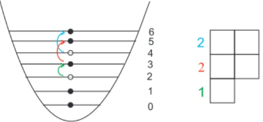
The number of D4 branes corresponds to the rank N of the gauge group, and the chemical potentials of D2 and D0 branes are identified with a combination of the theta angle and the gauge coupling of the Yang–Mills theory. In the large N limit, there is a chiral factorization of the partition function of 2-dimensional U(N) Yang-Mills,. According to the Fermi-Dirac distribution, the free fermion partition function for the N-fermion is the canonical ensemble.
The topological string splitting function, however, corresponds to a fermi sea with an arbitrary number of excitations on the fermi surface and the same number. For N → ∞, the excitations occur only at the fermi sea surfaces, since excitations within the sea are suppressed by e−N. When we consider finite N, the previous factorization is not correct as there are overcounts - the double counting of a fermion excitation on the upper and lower surfaces of the fermi sea.
Second approach to handling non-perturbative correctionscorrections
Gromov-Witten invariants
Now we want to extract the Gromov-Witten invariants of the modified topological partition function of the set Ψ. It has the nice property that the free energy of the topological set is convergent in every genus. There is no explicit form for Gromov-Witten invariants; however, Paul Cook wrote mathematica code [32] to calculate these numbers.
We can extract the Gromov-Witten invariants from that paper and find that they successfully match our results.
Modularity and holomorphicity
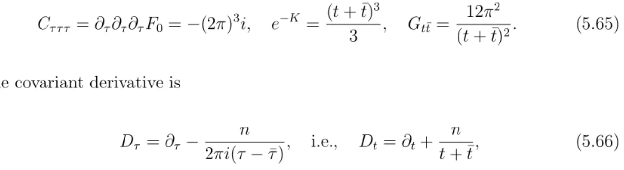
For true polarization, the amplitudes of the Fg strings will be holomorphic but quasimodular; for holomorphic, Fgis is modular but not fully holomorphic. In order to satisfy the holomorphic anomaly equation, we must use a modular form for each amplitude of the topological genus set. ˆFg is a modular form of weight 6g-6, so it turns out to be a covariant derivative with respect to t.
When solving the holomorphic anomaly equation, we find that C1(2) = 1. The derivative with respect to the modulus can be changed to the derivative with respect to ˆE2 by the chain rule,. A possible reason is that we need to choose a holomorphic polarization to use the holomorphic anomaly equation and then change the polarization to a true polarization by transforming E2(τ) to ˆE2(τ,τ¯) to obtain a modular form. Here, the periods we calculate are on some non-compact cycles, and the result is somewhat ambiguous, which means that the polarization we chose may not be holomorphic.
Summary and Open Questions
Low genus/boundary topological string holo- morphic equation
For the right-hand side, ∂x∂j∂x2 k contains two terms, where the two derivatives act on the same term in W or on different terms in W .
New approach to factorize Yang-Mills parti- tion functiontion function
- Topological string side
- Yang-Mills side
Now we want to prove the recursive relation between our newly defined function Ψ and the topological string partition function ψ. By shifting the variable in the first product by p → p−k and the one in the second product by p→p−(N+k), it becomes. This series is absolutely convergent to a holomorphic function ofτ in the upper half-plane. the Eisenstein series changes as G2k.