The Structure of Regional Original Revenue and Its Effect on Economic Growth: Facts from Regencies and Cities in Central Jawa
Wahyudi Susanto1 Catur Sugiyanto2
Gadjah Mada University - Indonesia Abstract
This study aims to determine the structure of Regional Original Revenue (PAD) in its effect on economic growth. The data used are panel data from 35 regencies and cities in Central Java for the period 2005 to 2015. Data are taken from the Regencies and Cities Financial Audit Results Reports in Central Java. Data analysis technique uses Panel Vector Error Correction Model (PVECM) and Panel Granger Causality Test to determine the relationship between economic growth and PAD components, namely regional tax revenue, regional retribution revenue, regional wealth revenue and other legitimate revenue. The results of this study found a one-way causality relationship from tax revenue to economic growth. There is a two-way relationship occurs between retribution revenue and economic growth. There is a one-way relationship from the regional wealth revenue to economic growth. There is a one-way relationship from the total regional original revenue (PAD) to economic growth. There is no relationship between other legitimate revenue and economic growth. In the short run, the economic growth over a given period was positively and significantly affected by the tax revenue, retribution revenue and regional original revenue (PAD) of the previous year, while regional wealth revenue has a negative and significant affect on economic growth. In the long run, tax revenue, retribution revenue and regional original revenue (PAD) affect by positively and significantly to economic growth, while regional wealth revenue has a negative and significant affect on economic growth.
Keywords: Regional Original Revenue (PAD), Economic Growth, Granger Causality Test, Panel Vector Error Correction Model (PVECM).
1 Wahyudi Susanto is a Student of Master of Economics of Development Program, Faculty of Economics and Business, Gadjah Mada University. E-mail: [email protected]
2 Catur Sugianto is a Lecturer of Master of Economics of Development Program, Faculty of Economics and Business, Gadjah Mada University. E-mail: [email protected]
The Structure of Regional Original Revenue and Its Affect on Economic Growth: Facts from Regencies and Cities in Central
Jawa
Wahyudi Susanto and Catur Sugiyanto
I. Introduction
Based on MPR Decree No. XV/MPR/1998 dated January 1, 2001 the Government of the Republic of Indonesia officially declared the commencement of the implementation of regional autonomy. Regional autonomy based on Law Number 22 of 1999 is more of a decentralized nuance, in which regions are close as separate autonomous regions, which use the central government delegated to the governor.
Fiscal decentralization is the delegation of authority to the regions to manage their own financial resources, so that regions have more opportunities to regulate their households. The basic principle of implementing fiscal decentralization in Indonesia is "Money Follows Functions", which is the main function of public services delivered, by submitting sources of revenue to the regions (Siagian 2010, 3).
The sources of regional revenue in the form of Regional Original Revenue (PAD) and transfers (General Allocation Funds, Revenue Sharing Funds, Special Allocation Funds and Autonomy Funds) are expected to increase economic growth and improve the welfare of people in the area. Economic growth is an increase in revenue to the amount of the value of goods and services produced by an economy within one year (Hubbard dkk. 2014, 32).
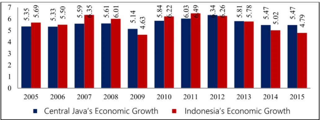
Figure 1. Comparison of Central Java's Economic Growth with Indonesia
Source: Berita Resmi Statistik BPS, 2017
Economic growth in Central Java averages 5,47% and is always below national economic growth in the 2005-2010 period. In the 2011-2015 period, the opposite applies, economic growth in Central Java on average remained at
5.35 5.33 5.59 5.61 5.14 5.84 6.03 6.34 5.81 5.47 5.475.69 5.50 6.35 6.01 4.63 6.22 6.49 6.26 5.78 5.02 4.79
0 1 2 3 4 5 6 7
2005 2006 2007 2008 2009 2010 2011 2012 2013 2014 2015 Pertumbuhan Ekonomi JatengCentral Java’s Economic Growth Pertumbuhan Ekonomi IndonesiaIndonesia’s Economic Growth
5,82% as shown in Figure 1. This indicates that economic growth in Central Java is able to sustain national economic growth.
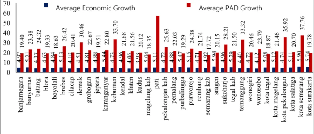
Figure 2. Comparison of Central Java's economic growth with PAD growth in regencies and cities in Central Java
Source: Official Publication of BPS and BPK, 2017
Factors that foster the economy include ownership of natural resources, people population, labor and technology. The economy of the Central Java region is interrelated because of the transportation system. Therefore, an analysis of the relationship between PAD and regional economic growth in Central Java must be done by panel analysis.
In Figure 2, economic growth in regencies and cities in Central Java is relatively stable on average at 4,90% in the period 2005-2015. PAD growth is relatively fluctuating and on average is always above economic growth, which is 24%. Based on this, it seems that PAD has nothing to do with economic growth.
An empirical study of the relationship between tax and economic growth is still not conclusive. Some studies prove the positive affect of tax on economic growth including Easterly and Rebelo (1993), Iimi (2005), Arnold (2008), Hammond and Tosun (2009), Myles (2009), Xing (2011), Bacarreza, Vazquez, and Vulovic (2013), Bujang, Hakim, and Ahmad (2013), Stoilova and Patonov (2013), Szarowska (2013), Devkota (2014), Mutiara (2015), Takumah and Iyke (2015), Saidin, Basit, and Hamza (2016), as well as Stoilova (2017). Studies that proves the positive affect of tax on economic growth states that increasing tax revenues will directly increase government revenues.
On the other hand, other researchers also prove the negative affect of tax on economic growth including Sugiyanto (1995), Davoodi and Zou (1998), Kneller, Bleaney, and Gemmell (1999), Widmalm (2001), Folster and Henrekson (2001), Lee and Gordon (2004), Bodman, Heaton, and Hodge (2009), Pose and Krøijer (2009), Pose and Ezcurra (2010), Gemmell, Kneller, and Sanz (2013),
4.97 5.21 4.37 4.63 4.84 5.13 4.10 4.51 4.81 4.88 5.44 4.73 4.96 4.06 3.93 5.04 5.11 4.72 4.88 5.47 5.15 4.71 4.92 5.94 4.96 5.29 4.40 4.72 4.12 5.08 5.12 4.74 5.11 5.90 5.74
19.40 23.38 24.32 19.33 18.63 26.42 20.41 30.46 22.67 19.51 22.80 33.70 21.68 21.56 20.12 18.35
61.62
25.63 22.03 19.29 24.38 21.74 17.72 20.15 28.21 21.50 33.32 20.46 23.79 18.87 21.46 35.92 20.70 37.76 19.78
0 10 20 30 40 50 60 70
banjarnegara banyumas batang blora boyolali brebes cilacap demak grobogan jepara karanganyar kebumen kendal
klaten kudus magelang kab pati pekalongan kab pemalang purbalingga purworejo rembang semarang kab sragen sukoharjo tegal kab temanggung wonogiri wonosobo kota tegal kota magelang kota pekalongan kota salatiga kota semarang kota surakarta
Rerata Pertumbuhan EkonomiAverage Economic Growth Rerata Pertumbuhan PADAverage PAD Growth
Anicic, Jelic, and Durovic (2015), Paparas and Richter (2015), Yushkov (2015) and Vatamanu and Oprea (2017). Studies that proves the negative affect of tax on economic growth states that relatively high taxes will reduce public consumption and investment.
Studies that state a negative relationship between economic growth and tax are found by Taha, Loganathan, and Colombage (2011) and Triastuti and Pratomo (2016). These studies state that economic growth is increasing because of reduced tax collection on the community which causes the level of consumption and investment to rise, thus increasing GDP.
Retribution is proven to encourage economic growth because the function of retribution is one source of regional revenue that can be used for regional government spending which can increase GDP as the study results of Mutiara (2015) and Pattawe et al. (2017). Studies that shows that retribution has a negative effect on economic growth has not been found.
PAD is encouraging economic growth because PAD functions as one of the fiscal components of regional governments in equitable distribution of regional development and equitable distribution of revenue for local communities so as to facilitate economic activities and consumption that can increase GDP as studies result of Putri (2015), Hendriwiyanto (2016), Rori, Luntungan, and Niode (2016), Manek and Badrudin (2016) and Muti'ah (2017).
On the other hand, studies that found a positive relationship of economic growth to PAD include Desmawati, Zamzani, and Zulgani (2015) and Susanti et al. (2017).
Economic growth and PAD are two key variables in the region.
However, the relationship between the two variables is still not conclusive. On the one hand, the revenue of PAD is an engine that drives investment so that it can encourage economic growth. Similarly, economic growth is a source of PAD.
On the other hand, PAD is also negative because the high revenue of PAD causes public consumption and investment to decline, while economic growth has a negative effect on PAD given the ineffectiveness of regional government spending in facilitating economic activity.
With the above conditions it is still unclear how the nature of the relationship between PAD and economic growth in Central Java Province. By knowing the conditions of the relationship between the PAD structure and economic growth, the Regional Government can formulate fiscal policies that will be taken to increase PAD and economic growth in Central Java.
Economic growth, taxes, retribution, regional wealth, other legitimate revenue and PAD are believed to be interrelated economic variables. However, the literature shows empirical differences in how the style of tax relations (as a
source of PAD) with economic growth. Meanwhile, data on economic growth and PAD in Central Java seems unrelated during the period 2005-2015.
This study aims to determine the relationship between PAD and economic growth in regencies and cities in Central Java. The findings of this study are expected to help regional governments improve understanding of the nature of PAD relations and economic growth and take fiscal policies to maximize the PAD of their respective regions to advance the economy in their regions.
II. Literature Review
2.1. Regional Government Original Revenue System in Indonesia
Tax according to Law Number 28 of 2007 concerning Third Amendment to Law Number 6 of 1983 concerning General Provisions and Tax Procedures is a mandatory contribution to the state which is owed by an individual or an entity that is compulsory under the law, with no direct compensation and is used for the state's needs as much as possible for the people's prosperity.
Regional taxes consist of, among others, hotel tax, restaurant tax, entertainment tax, advertisement tax, street lighting tax, parking tax, groundwater tax, land and building tax, land acquisition rights and building tax.
The central government has again issued regulations on regional taxes and regional retribution through Law Number 28 of 2009.
With this Law, Law Number 18 of 1997 was revoked as amended by Law Number 34 of 2000. Regional retribution includes, retribution on public services, cleaning services, funeral services, roadside parking, land rent, tera test, business service fees, terminals, licensing levies, permission to disturb and others.
Law Number 33 of 2004 classifies the types of results of regional wealth management that are separated, broken down according to the revenue object which includes part of the return on equity participation in Regional Owned Enterprises (BUMD), part of the return on equity participation in State Owned Enterprises (BUMN) and the return equity participation in privately owned companies or community groups. Among other legitimate revenue is the sale of unregistered regional wealth, the results of the utilization or utilization of regional assets that are not separated, current account services, interest revenue, compensation claims, profit from the difference between the rupiah exchange rate against foreign currencies and commissions, deductions or other forms as a result of the sale and / or procurement of goods and or services by the region.
According to Law Number 17 of 2003 Article 1 Letter 9 and Article 11 Paragraph 3 concerning State Finance, state revenues are all cash receipts that enter the state consisting of tax revenues and not taxes and grants. Tax revenue
is also classified into two, namely tax revenue from the central and tax revenue from the region.
Regional tax revenues are cash receipts that go into the regional treasury collected by the regional government (in this case carried out by the Regional Revenue Service/Dispenda) which are used to finance the households of the regional government and are listed in the Regional Revenue and Expenditure Budget (APBD).
2.2. Economic growth
Understanding economic growth according to Todaro (2006, 45) is a process that causes changes in people's lives, namely political changes, social structures, social values and the structure of their economic activities. In addition, according to Arsyad (1997, 57) economic growth is a process that causes an increase in the per capita revenue of a country's population in the long run accompanied by an improvement in the institutional system.
Economic growth is often measured using growth of Gross Domestic Product (GDB/GRDB). Gross Regional Domestic Product (GRDP) basically is the amount of added value produced by all business units in a particular area, or is the sum of the value of the final goods and services produced by all economic units. Hubbard et al. (2014, 72) states that calculating real GDP uses a comparison of the year to base year and uses the base year price as the basis for calculating the value of goods and services during the calculated annual period.
2.3. Relationship between PAD and economic growth
According to Saragih (2003, 15), an increase in PAD is actually an excess of regional economic growth whose positive economic growth is likely to get an increase in PAD. This perspective should make regional governments more concentrated on empowering local economic forces to create economic growth rather than simply issuing regulatory products related to taxes or retribution.
Increasing the economic growth of a region is also able to attract investors to invest in the region so that the sources of PAD, especially those from regional taxes, will increase. High PAD can then be used by regional governments to provide adequate public services so that this will increase capital expenditure. Such spending will increase aggregate expenditure and enhance economic activity.
As economic activity increases, the flow of government revenues through PAD also increases. Government expenditure reflects government policies to improve people's welfare. The government must provide public goods, because there is no private sector that wants to provide goods that people enjoy. Government activities will shift from providing facilities to expenditures for social activities which can ultimately increase economic activity.
In this case, the regional government imposes regional tax and retribution so that PAD also increases.
III. Method
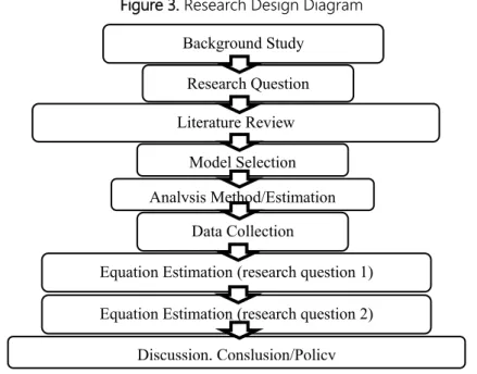
To make it easier to understand the strategy of this research, it can be described the following research design flowchart.
Figure 3. Research Design Diagram
The data used in this study are panel data for the years 2005 to 2015 that are sourced from the Audit Report on the Financial Statements of Regencies and Cities Governments in Central Java that issued by the Republic of Indonesia Supreme Audit Agency.
According to Granger (1969), causality can be divided into two, namely long run and short run. Sims (1972), developed the VAR method to estimate short run and long run relationships between variables which can be formulated as follows:
𝑦𝑦𝑖𝑖𝑖𝑖=𝛼𝛼𝑖𝑖 +𝛽𝛽₁ 𝑦𝑦𝑖𝑖𝑖𝑖−1+. . . … . . + 𝛽𝛽𝑘𝑘𝑦𝑦𝑖𝑖𝑖𝑖−𝑘𝑘+ 𝜖𝜖𝑖𝑖𝑖𝑖 (1) The model's initial equation is assumed to be a PVAR model used to describe the following causality relationships:
𝑌𝑌𝑖𝑖𝑖𝑖 = 𝛼𝛼₀+ 𝛼𝛼₁ 𝑌𝑌𝑖𝑖𝑖𝑖−1 +𝛼𝛼₂ 𝑌𝑌𝑖𝑖𝑖𝑖−𝑛𝑛 +𝛽𝛽₁ 𝑋𝑋𝑖𝑖𝑖𝑖−1+𝛽𝛽₂ 𝑋𝑋𝑖𝑖𝑖𝑖−𝑛𝑛+ µ𝑖𝑖𝑖𝑖 (2) 𝑋𝑋𝑖𝑖𝑖𝑖 = 𝛾𝛾₀+ 𝛾𝛾₁ 𝑋𝑋𝑖𝑖𝑖𝑖−1 + 𝛾𝛾₂ 𝑋𝑋𝑖𝑖𝑖𝑖−𝑛𝑛 +𝛿𝛿₁ 𝑌𝑌𝑖𝑖𝑖𝑖−1+𝛿𝛿₂ 𝑌𝑌𝑖𝑖𝑖𝑖−𝑛𝑛+ 𝑣𝑣𝑖𝑖𝑖𝑖 (3) where: Y = endogenous variable 1; X = endogenous variable 2.
Research Question Literature Review
Model Selection
Data Collection
Equation Estimation (research question 1) Equation Estimation (research question 2)
Discussion, Conslusion/Policy Analysis Method/Estimation
Background Study
Panel Vector Auto Regression (PVAR) and Panel Vector Error Correction Model (PVECM)
According to Dorsman et al. (2012), causality can be explained by the PVAR model at level I(1). Granger Causality Test can be done with the PVAR model by separating exogenity from the Wald Test. Long run relationships can be investigated using the Panel Vector Error Correction Model (PVECM) and the affect of short run relationships using the Wald Test. Use PVECM if the data form is not stationary at I(0) and cointegration occurs even though it is stationary at I(1). PVECM can restructure the long run relationship of endogenous variables in order to remain convergent into their cointegration relationship. The PVECM equation can be formulated as follows:
∆𝑦𝑦𝑖𝑖𝑖𝑖 =𝛿𝛿𝛿𝛿𝑖𝑖𝑖𝑖 +𝛼𝛼𝛽𝛽₁ 𝑦𝑦𝑖𝑖𝑖𝑖−1+𝛤𝛤𝛤𝛤𝑖𝑖𝑖𝑖+ 𝜖𝜖𝑖𝑖𝑖𝑖 , t= 1,2,3,…T (4) where: ∆𝑦𝑦𝑖𝑖𝑖𝑖= matrix difference k observed variable; 𝑦𝑦𝑖𝑖𝑖𝑖−1= matrix first lag observed variable; 𝛿𝛿= parameter matrix of the model determinant component;
𝛿𝛿𝑖𝑖𝑖𝑖 = vector determinant component to t; 𝛼𝛼𝛽𝛽₁ = long-run equation coefficient
matrix; 𝛤𝛤 = dynamic matrix of short-run equations; 𝛤𝛤𝑖𝑖𝑖𝑖= matrix difference observed in lag k; 𝜖𝜖𝑖𝑖𝑖𝑖= matriks error term.
Granger Causality Test
This study will examine the direction of the relationship between economic growth variables with interest variables namely tax revenue, retribution revenue, regional wealth revenue, other legitimate revenue and PAD.
Bernard and Willet (1996) state that there are at least two methods for determining the direction of relationships between variables. First, by testing causality statistically using the Granger Test. Second, by determining the direction of relations on an ad hoc basis based on the characteristics of the conditions formed, namely by looking at whether economic growth is often caused by changes in interest variables or interest variables more often caused by economic growth.
IV. Results and Discussion
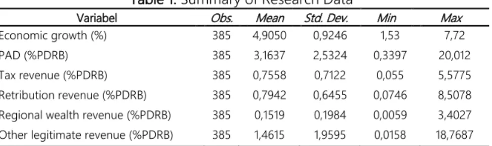
To facilitate the analysis and interpretation, the data analyzed will all be made into a percentage of the nominal real GDP of each region. Observation data analyzed amounted to 385 consisting of 35 regencies and cities in the 11- year period (2005-2015). The following is a summary table of data that will be used in the research analysis:
Table 1. Summary of Research Data
Variabel Obs. Mean Std. Dev. Min Max
Economic growth (%) 385 4,9050 0,9246 1,53 7,72
PAD (%PDRB) 385 3,1637 2,5324 0,3397 20,012
Tax revenue (%PDRB) 385 0,7558 0,7122 0,055 5,5775
Retribution revenue (%PDRB) 385 0,7942 0,6455 0,0746 8,5078 Regional wealth revenue (%PDRB) 385 0,1519 0,1984 0,0059 3,4027 Other legitimate revenue (%PDRB) 385 1,4615 1,9595 0,0158 18,7687 Source: LHP-LKPD, be treated (BPK 2005-2015)
1. Stationarity test
As a first step in data analysis, it is necessary to do a unit root test on variables that are important variables in this study, namely economic growth variables, tax revenue, retribution revenue, regional wealth revenue, other legitimate revenue and PAD variables. Unit root testing uses the Augmented Dickey-Fuller Test (ADF) and Levine-Liu-Chu Test methods. The data is said to be stationary if the statistical test value is smaller than the critical value of at least 5% which is equal to -2,8671 and the probability value is smaller than 0,05.
Data on economic growth at I(0) or data at the level indicates that there is no unit root because the statistical test value is -4,6292 and smaller than the critical level of 1% (-3,4433), so the data is said to be stationary. Data other than economic growth variables have unit roots because the test value is at a value greater than -2,8671. With these results, it is necessary to see first different level of PAD data, tax revenue, retribution revenue, regional wealth revenue, other legitimate revenue there are still units root or not.
Data testing shows that all data have no root units with statistical values greater than the critical level of 1% (-3,4443). So it can be concluded that all data to be used in this study are stationary at I(1). Granger and Newbold (1974), say that the non-stationary data will produce variable relationships that look statistically significant but in reality it is not or the relationship is not as big as the regression produced.
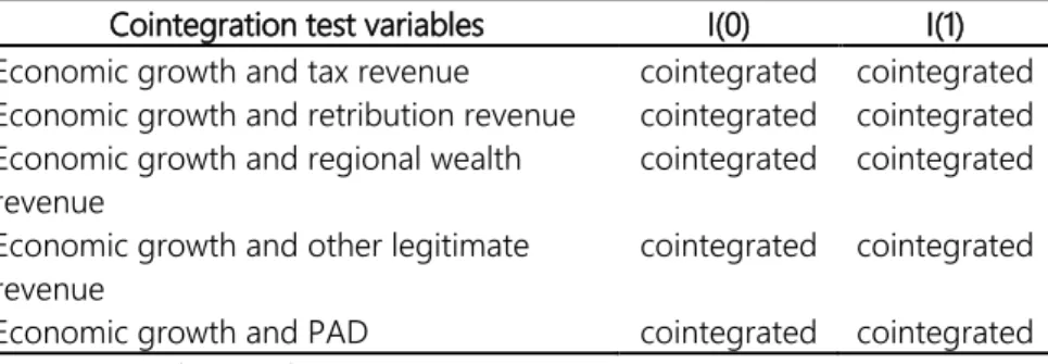
2. Cointegration test
Cointegration testing is used to determine the balance relationship intervariables in the long-run, in this case is the variable of economic growth and PAD. Cointegration testing using the Pedroni Residual Cointegration Test method is by comparing the probability values of seven panel categories. The seven panel categories are v-statistics panel, rho-statistics panel, PP-statistics panel, ADF-statistics panel, rho-statistical group, PP-statistical group and ADF- statistical group. If the probability value of the seven criteria is smaller than 0.05, the null hypothesis that economic growth and PAD do not have cointegration
cannot be rejected. Conversely, if the probability value is greater than 0.05, the null hypothesis can be rejected.
Table 2. Cointegration Test Results Using Pedroni Residual Cointegration Test at I(0) and I(1)
Cointegration test variables I(0) I(1) Economic growth and tax revenue cointegrated cointegrated Economic growth and retribution revenue cointegrated cointegrated Economic growth and regional wealth
revenue cointegrated cointegrated
Economic growth and other legitimate
revenue cointegrated cointegrated
Economic growth and PAD cointegrated cointegrated
Source: LHP-LKPD, be treated (BPK 2005-2015)
The test results in Table 2, cointegration occurs in both testing models on data level/I(0) and at I(1). Therefore, the analysis continued with PVECM. This is because both variables occur long run relationships, while PVAR requires that no cointegration between variables will be estimated.
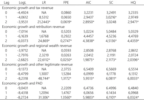
3. Optimal lag selection
According to Amri (2017), the optimal choice of lag is used to determine the time period of the influence of a variable on other variables optimally.
Knowledge of optimal lag is due to the affect of changing a variable on other variables does not always occur in the same time period.
Table 3. Optimal Lag Selection Results
Lag LogL LR FPE AIC SC HQ
Economic growth and tax revenue
0 -4,4924 NA 0,0860 3,2231 3,2491 3,2335
1 -4,0612 8,5312 0,0650 2,9437 3,0216* 2,9749
2 -3,9531 21,2443* 0,0619* 2,8950* 3,0248 2,9471*
Economic growth and retribution revenue
0 -7,0114 NA 0,5203 5,0224 5,0484 5,0329
1 -6,1639 1,6768 0,2922 4,4457 4,5236 4,4769
2 -6,0373 24,869* 0,2747* 4,3838* 4,5136* 4,4359*
Economic growth and regional wealth revenue
0 -3,9712 NA 0,0593 2,8508 2,8768 2,8612
1 -2,7976 2,3219 0,0263 2,0412 2,1191 2,0724
2 -2,6825 22,6112* 0,0250* 1,9875* 2,1173* 2,0396*
Economic growth and other legitimate revenue
0 -9,1373 NA 2,3755 6,5409 6,5669 6,5514
1 -8,4799 1,3007 1,5284 6,0999 6,1778 6,1312
2 -8,2318 48,744* 1,3172* 5,9513* 6,0811* 6,0033*
Economic growth and PAD
0 -9,0431 NA 2,2209 6,4736 6.4996 6,4840
1 -8,4318 1,2094 1,4767 6,0656 6.1434 6,0968
2 -8,2724 31.306* 1.3560* 5,9803* 6,1101* 6,0324*
Source: LHP-LKPD, be treated (BPK 2005-2015)
According to Table 3, it can be seen that the optimal lag choice is at the 2-year time horizon produced by LR test statistics, Final Predictor Error (FPE), Akaike Information Criteria (AIC), Schwarz Information Criteria (SIC) and Hannan-Quinn Information Criteria ( HQ). The optimal lag selection will use the optimal lag at the 2-year time horizon because it takes into account a closer time period so that it is possible to give an influence between the more optimal variables.
4. PVECM Analysis
The PVECM estimation can explain the long run and short run affects between variables. If previously the proposed equation model is PVAR with formulations as in equations (2) and (3), with the change in the estimation model from PVAR to PVECM, then the equation in the model can be written in the following formulation:
∆𝑌𝑌𝑖𝑖𝑖𝑖 = 𝛼𝛼1,𝑖𝑖+ 𝜑𝜑1,𝑖𝑖 𝐸𝐸𝐸𝐸𝐸𝐸𝑖𝑖,𝑖𝑖−1 +𝛴𝛴𝑗𝑗=1𝛶𝛶1,𝑗𝑗,𝑖𝑖 ∆𝑌𝑌𝑖𝑖,𝑖𝑖−𝑗𝑗+𝛴𝛴𝑗𝑗=1 𝜃𝜃1,𝑗𝑗,𝑖𝑖 ∆𝑋𝑋𝑖𝑖,𝑖𝑖−𝑗𝑗+ µ1,𝑖𝑖𝑖𝑖 (5)
∆𝑋𝑋𝑖𝑖𝑖𝑖 = 𝛼𝛼2,𝑖𝑖+ 𝜑𝜑2,𝑖𝑖 𝐸𝐸𝐸𝐸𝐸𝐸𝑖𝑖,𝑖𝑖−1 +𝛴𝛴𝑗𝑗=2𝛶𝛶2,𝑗𝑗,𝑖𝑖 ∆𝑌𝑌𝑖𝑖,𝑖𝑖−𝑗𝑗+𝛴𝛴𝑗𝑗=2 𝜃𝜃2,𝑗𝑗,𝑖𝑖 ∆𝑋𝑋𝑖𝑖,𝑖𝑖−𝑗𝑗+ 𝜈𝜈1,𝑖𝑖𝑖𝑖 (6) where: i = regency/city; j = lag optimal; ECT = Error Correction Term obtained from the cointegration relationship 𝜃𝜃1and 𝜃𝜃2; Y = endogenous variable 1; X = endogenous variable 2.
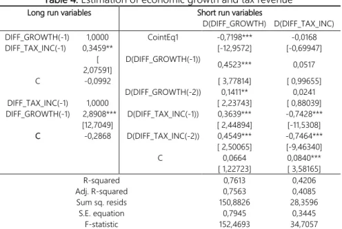
Economic growth and tax revenue. The estimation results shown in Table 4.4 show that in the long run the tax revenue can affect economic growth significantly at the 95% confidence level with a coefficient of 0,3459. That means, if tax revenue rises 1% of GRDP, it will increase economic growth by 0,3459%.
On the other hand, also occurs in the long run that economic growth has a significant affect on the 99% confidence level with a coefficient of 2,8908. That means, if economic growth rises by 1%, it will increase tax revenues by 2,8908%
of GRDP.
In short run relationships, tax revenue in the first lag significantly affect economic growth at a 99% confidence level with a coefficient of 0,3639. That means, if the tax revenue for the past period increased by 1% of GRDP, it would increase economic growth by 0,3639% at current period. Similarly, in the second lag, the coefficient of tax revenue is 0,4549, which means that if the tax revenue of the past two periods increased by 1% of GRDP, it would increase economic growth by 0,4549%. Short run relationship tax revenue variable is also significantly affected by itself with a coefficient of 0,7428 in the first lag and 0,7464 in the second lag. That is, tax revenues affect economic growth on the other hand also affect themselves.
Table 4. Estimation of economic growth and tax revenue
Long run variables Short run variables
D(DIFF_GROWTH) D(DIFF_TAX_INC)
DIFF_GROWTH(-1) 1,0000 CointEq1 -0,7198*** -0,0168
DIFF_TAX_INC(-1) 0,3459** [-12,9572] [-0,69947]
2,07591] [ D(DIFF_GROWTH(-1)) 0,4523*** 0,0517
C -0,0992 [ 3,77814] [ 0,99655]
D(DIFF_GROWTH(-2)) 0,1411** 0,0241
DIFF_TAX_INC(-1) 1,0000 [ 2,23743] [ 0,88039]
DIFF_GROWTH(-1) 2,8908*** D(DIFF_TAX_INC(-1)) 0,3639*** -0,7428***
[12,7049] [ 2,44894] [-11,5308]
C -0,2868 D(DIFF_TAX_INC(-2)) 0,4549*** -0,7464***
[ 2,50065] [-9,46340]
C 0,0664 0,0840***
[ 1,22723] [ 3,58165]
R-squared 0,7613 0,4206
Adj. R-squared 0,7563 0,4085
Sum sq. resids 150,8826 28,3596
S.E. equation 0,7945 0,3445
F-statistic 152,4693 34,7057
Explanation: Number in [ ] is a t-statistic; *** significant at level 1%; ** significant at level 5%; * significant at level 10%.
Source: LHP-LKPD, be treated (BPK 2005-2015)
On the opposite relationship, namely economic growth with tax revenues found in the short run, but not significant for tax revenues. Economic growth in the short run is significant with a 99% confidence level in the first lag with a coefficient of 0,4523 and significant with a level of trust in the second lag with a coefficient of 0,1411.
The value of speed of adjustment coefficient of economic growth equation is -0,7198. That means, the adjustment of economic growth to return to equilibrium is quite fast. Coefficient -0,7198 shows that the equilibrium adjustment of economic growth in the past period will be corrected by 71,98%
in the current period. On the other hand, the value of coefficient of tax revenue is not significant, meaning that in the previous period there was no adjustment in tax revenue to return to equilibrium at current period.
Based on the estimation results in Table 4, the short run equation model of economic growth and tax revenues are:
∆𝛿𝛿𝑑𝑑𝑑𝑑𝑑𝑑_ 𝑡𝑡𝑡𝑡𝑡𝑡_𝑑𝑑𝑖𝑖𝑖𝑖𝑖𝑖𝑖𝑖 = −0,0168 (𝛿𝛿𝑑𝑑𝑑𝑑𝑑𝑑_𝑡𝑡𝑡𝑡𝑡𝑡_𝑑𝑑𝑖𝑖𝑖𝑖 𝑖𝑖𝑖𝑖−1+ 2,8908 𝛿𝛿𝑑𝑑𝑑𝑑𝑑𝑑_𝑔𝑔𝑔𝑔𝑔𝑔𝑔𝑔𝑡𝑡ℎ 𝑖𝑖𝑖𝑖−1 − 0,2868)−0,7428 ∆𝛿𝛿𝑑𝑑𝑑𝑑𝑑𝑑_𝑡𝑡𝑡𝑡𝑡𝑡_𝑑𝑑𝑖𝑖𝑖𝑖 𝑖𝑖𝑖𝑖−1 − 0,7464 ∆𝛿𝛿𝑑𝑑𝑑𝑑𝑑𝑑_𝑡𝑡𝑡𝑡𝑡𝑡_𝑑𝑑𝑖𝑖𝑖𝑖 𝑖𝑖𝑖𝑖−2 +
0,0517 ∆𝛿𝛿𝑑𝑑𝑑𝑑𝑑𝑑_𝑔𝑔𝑔𝑔𝑔𝑔𝑔𝑔𝑡𝑡ℎ 𝑖𝑖𝑖𝑖−1 + 0,0240 ∆𝛿𝛿𝑑𝑑𝑑𝑑𝑑𝑑_𝑔𝑔𝑔𝑔𝑔𝑔𝑔𝑔𝑡𝑡ℎ 𝑖𝑖𝑖𝑖−2+ 0,0840 (7)
∆𝛿𝛿𝑑𝑑𝑑𝑑𝑑𝑑_ 𝑔𝑔𝑔𝑔𝑔𝑔𝑔𝑔𝑡𝑡ℎ𝑖𝑖𝑖𝑖= −0,7198 (𝛿𝛿𝑑𝑑𝑑𝑑𝑑𝑑_𝑡𝑡𝑡𝑡𝑡𝑡_𝑑𝑑𝑖𝑖𝑖𝑖 𝑖𝑖𝑖𝑖−1+ 2,8908 𝛿𝛿𝑑𝑑𝑑𝑑𝑑𝑑_𝑔𝑔𝑔𝑔𝑔𝑔𝑔𝑔𝑡𝑡ℎ 𝑖𝑖𝑖𝑖−1 − 0,2868) + 0,3639 ∆𝛿𝛿𝑑𝑑𝑑𝑑𝑑𝑑_𝑡𝑡𝑡𝑡𝑡𝑡_𝑑𝑑𝑖𝑖𝑖𝑖 𝑖𝑖𝑖𝑖−1 + 0,4549 ∆𝛿𝛿𝑑𝑑𝑑𝑑𝑑𝑑_𝑡𝑡𝑡𝑡𝑡𝑡_𝑑𝑑𝑖𝑖𝑖𝑖 𝑖𝑖𝑖𝑖−2 + 0,4523 ∆𝛿𝛿𝑑𝑑𝑑𝑑𝑑𝑑_𝑔𝑔𝑔𝑔𝑔𝑔𝑔𝑔𝑡𝑡ℎ 𝑖𝑖𝑖𝑖−1 + 0,1411 ∆𝛿𝛿𝑑𝑑𝑑𝑑𝑑𝑑_𝑔𝑔𝑔𝑔𝑔𝑔𝑔𝑔𝑡𝑡ℎ 𝑖𝑖𝑖𝑖−2+ 0,664 (8)
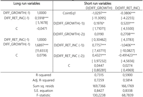
Economic growth and retribution revenue. The estimation results in Table 5 between the variables of economic growth and retribution revenue in the long run are retribution revenue can affect economic growth significantly at the 99% confidence level with a coefficient of 0,5918. That means, if the retribution revenue increases 1% of the GRDP, it will increase economic growth by 0,5918%. On the other hand, economic growth in the long run is also able to significantly affect retribution revenues at a 99% confidence level with a coefficient of 1,6897. That means, if economic growth rises 1%, it will increase retribution revenue by 1,6897% of GRDP.
Estimated short run relationship, retribution revenue affects economic growth significantly at the 99% confidence level with a coefficient of 0,7757 in the first lag. That means, retribution revenue in one previous period rose 1% of GRDP, will affect economic growth by 0,77% at current period. Similarly, in the second lag, retribution revenue affects economic growth significantly at the 99%
confidence level with a coefficient of 0,4321. That means, if the retribution revenue for the past two periods rose by 1% from the GRDP, it would increase economic growth at this time by 0,4321%. In addition, retribution revenue also has a significant affect on the 99% confidence level in the first lag and the second lag for itself with a coefficient value of -1,0405 in the first lag and -0,4914 in the second lag. That means, an increase in retribution revenue in one and two previous periods amounting to 1% of GRDP, will affect the decrease in retribution revenue by 1,0405% in the first lag and 0,4914% in the second lag.
The estimation results of economic growth on retribution revenue in the short run is that economic growth affects retribution revenue significantly at the 99% confidence level with a coefficient of 0,5200 in the first lag. That means, if economic growth in the previous period rose 1%, it would increase retribution revenue by 0,5200% of the current GRDP. In the second lag, economic growth also still affects retribution revenue significantly at the 99% confidence level with a coefficient of 0,2708. That means, if the economic growth of the previous two periods rose by 1%, it would increase the current retribution revenue by 0,2708%
from GRDP.
In estimating economic growth towards itself in the short run, it was found that the first lag economic growth was able to affect itself at 90%
confidence level with a coefficient of 0,1976. However, in the second lag economic growth has no significant affect on itself.
Value of speed of adjustment coefficient of economic growth equation is -1,0297. That means, adjusting economic growth to return to equilibrium very quickly. Coefficiency -1,0297 shows that the equilibrium adjustment of economic growth in the past period will be corrected by 102% in the current period.
Meanwhile, the value of speed of adjustment coefficient of retribution revenue is -0,3806. This shows that the adjustment of retribution revenue to return to
equilibrium is quite fast because the previous period's equilibrium will be corrected by 38,06% in the current period.
Table 5. Estimation of economic growth and retribution revenue
Long run variables Short run variables
D(DIFF_GROWTH) D(DIFF_RET_INC) DIFF_GROWTH(-1) 1,0000 CointEq1 -1,0297*** -0.3806***
DIFF_RET_INC(-1) 0,5918*** [-11.3095] [-4.2255]
[ 5,1678] D(DIFF_GROWTH(-1)) 0,1976* 0,5201***
C -0,0471 [ 1,71071] [ 4,5500]
D(DIFF_GROWTH(-2)) 0,0190 0,2708***
DIFF_RET_INC(-1) 1,0000 [ 0,30462] [ 4,3783]
DIFF_GROWTH(-1) 1,6897*** D(DIFF_RET_INC (-1)) 0,7757*** -1,0406***
[11,6553] [ 7,43711] [-10,0827]
C 0,0796 D(DIFF_RET_INC (-2)) 0,4321*** -0.491423***
[ 3,97232] [-4,5656]
C 0,0447 0,0274
[ 0,80281] [ 0,4969]
R-squared 0,7315 0,5900
Adj. R-squared 0,7259 0,5814
Sum sq. resids 169,7366 166,1769
S.E. equation 0,8427 0,8338
F-statistic 130,2238 68,7839
Explanation: Number in [ ] is a t-statistic; *** significant at level 1%; ** significant at level 5%; * significant at level 10%.
Source: LHP-LKPD, be treated (BPK 2005-2015)
Based on the estimation results in Table 5, the short run equation model of economic growth and retribution revenue are:
∆𝛿𝛿𝑑𝑑𝑑𝑑𝑑𝑑 𝑔𝑔𝑟𝑟𝑡𝑡𝑖𝑖𝑛𝑛𝑖𝑖𝑖𝑖𝑖𝑖=
−0,3806 (𝛿𝛿𝑑𝑑𝑑𝑑𝑑𝑑_𝑔𝑔𝑟𝑟𝑡𝑡_𝑑𝑑𝑖𝑖𝑖𝑖 𝑖𝑖𝑖𝑖−1+ 1,6897 𝛿𝛿𝑑𝑑𝑑𝑑𝑑𝑑_𝑔𝑔𝑔𝑔𝑔𝑔𝑔𝑔𝑡𝑡ℎ 𝑖𝑖𝑖𝑖−1−0,0796)− 1,0405 ∆𝛿𝛿𝑑𝑑𝑑𝑑𝑑𝑑_𝑔𝑔𝑟𝑟𝑡𝑡_𝑑𝑑𝑖𝑖𝑖𝑖 𝑖𝑖𝑖𝑖−1 − 0,4914 ∆𝛿𝛿𝑑𝑑𝑑𝑑𝑑𝑑_𝑔𝑔𝑟𝑟𝑡𝑡_𝑑𝑑𝑖𝑖𝑖𝑖 𝑖𝑖𝑖𝑖−2 +
0,5200 ∆𝛿𝛿𝑑𝑑𝑑𝑑𝑑𝑑_𝑔𝑔𝑔𝑔𝑔𝑔𝑔𝑔𝑡𝑡ℎ 𝑖𝑖𝑖𝑖−1 + 0,2708 ∆𝛿𝛿𝑑𝑑𝑑𝑑𝑑𝑑_𝑔𝑔𝑔𝑔𝑔𝑔𝑔𝑔𝑡𝑡ℎ 𝑖𝑖𝑖𝑖−2+ 0,0273 (9)
∆𝛿𝛿𝑑𝑑𝑑𝑑𝑑𝑑 𝑔𝑔𝑔𝑔𝑔𝑔𝑔𝑔𝑡𝑡ℎ𝑖𝑖𝑖𝑖=
−1,0297 (𝛿𝛿𝑑𝑑𝑑𝑑𝑑𝑑_𝑔𝑔𝑟𝑟𝑡𝑡_𝑑𝑑𝑖𝑖𝑖𝑖 𝑖𝑖𝑖𝑖−1+ 1,6897 𝛿𝛿𝑑𝑑𝑑𝑑𝑑𝑑_𝑔𝑔𝑔𝑔𝑔𝑔𝑔𝑔𝑡𝑡ℎ 𝑖𝑖𝑖𝑖−1−0,0796) + 0,7757 ∆𝛿𝛿𝑑𝑑𝑑𝑑𝑑𝑑_𝑔𝑔𝑟𝑟𝑡𝑡_𝑑𝑑𝑖𝑖𝑖𝑖 𝑖𝑖𝑖𝑖−1 + 0,4321 ∆𝛿𝛿𝑑𝑑𝑑𝑑𝑑𝑑_𝑔𝑔𝑟𝑟𝑡𝑡_𝑑𝑑𝑖𝑖𝑖𝑖 𝑖𝑖𝑖𝑖−2 +
0,1976 ∆𝛿𝛿𝑑𝑑𝑑𝑑𝑑𝑑_𝑔𝑔𝑔𝑔𝑔𝑔𝑔𝑔𝑡𝑡ℎ 𝑖𝑖𝑖𝑖−1 + 0,0190 ∆𝛿𝛿𝑑𝑑𝑑𝑑𝑑𝑑_𝑔𝑔𝑔𝑔𝑔𝑔𝑔𝑔𝑡𝑡ℎ 𝑖𝑖𝑖𝑖−2+ 0,0466 (10)
Economic growth and regional wealth revenue. The estimation result in Table 6 between economic growth and regional wealth revenue is the economic growth has a significant affect on regional wealth revenue at 99% confidence level with a coefficient of -1,7921. That means, in the long run, the economic growth of 1%, will reduce regional wealth revenue by 1,7921% of GDRP. In contrary, regional wealth revenue do not significantly affects economic growth in the long run.
In the short run, economic growth has a significant affect on regional wealth revenue in the first lag. At a 90% confidence level, the value of coefficient of economic growth is -0,0679. That means, if the economic growth rose by 1%, will decrease regional wealth revenue by 0,06% of GDRP. Meanwhile, in the second lag, economic growth has no significant affect on regional wealth revenue. In addition to affecting regional wealth revenue, economic growth also affects itself in the first lag at 99% confidence level with 0,4504 and in the second lag at 95% confidence level with coefficient of 0,1361.
The estimation of the affect of regional wealth revenue on economic growth is found that regional wealth revenue has a significant affect on economic growth at a 99% confidence level with a coefficient of -1,1328 in the first lag. In the second lag, regional wealth revenue has a significant affect on economic growth at a 95% confidence level with a coefficient of -1,2207. That means, if the regional wealth revenue in the previous period rose by 1%, will reduce economic growth by 1,1328% and in the previous two periods reduce economic growth by 1,2207% at current period. The affect of regional revenue wealth on itself is significant at the 99% confidence level in the first lag and the second lag. The coefficient on the first lag is -1,7676 and in the second lag is - 1,0770. This means that current regional wealth revenues will decrease by - 1,7676% of GRDP if regional wealth revenue in the previous period rises by 1%
from GRDP. Likewise, if in the previous two periods regional revenue has increased by 1% of GDRP, it would have caused a decrease in revenue of regional wealth by -1,0770% of current GRDP.
The coefficient of speed of adjustment of economic growth is 1,1624.
That means, economic growth to return to equilibrium is very quickly. 1,1624 coefficient which shows the economic equilibrium growth for the period to be corrected by -116% in the current period. Meanwhile, the coefficient of speed of adjustment of regional wealth revenue is -0,0479. This shows that the adjustment of regional wealth revenue to return to equilibrium is quite slow because the previous period's equilibrium will be corrected by 4,79% in the current period so that it takes 20 periods to reach equilibrium.
Based on the results in Table 6, the short run equation model of economic growth and regional revenue are:
∆𝛿𝛿𝑑𝑑𝑑𝑑𝑑𝑑_ 𝑔𝑔𝑑𝑑𝑖𝑖ℎ_𝑑𝑑𝑖𝑖𝑖𝑖𝑖𝑖𝑖𝑖= −0,0479 (𝛿𝛿𝑑𝑑𝑑𝑑𝑑𝑑_𝑔𝑔𝑑𝑑𝑖𝑖ℎ_𝑑𝑑𝑖𝑖𝑖𝑖 𝑖𝑖𝑖𝑖−1−1,7921 𝛿𝛿𝑑𝑑𝑑𝑑𝑑𝑑_𝑔𝑔𝑔𝑔𝑔𝑔𝑔𝑔𝑡𝑡ℎ 𝑖𝑖𝑖𝑖−1+ 0,0520)−1,7675 ∆𝛿𝛿𝑑𝑑𝑑𝑑𝑑𝑑_𝑔𝑔𝑑𝑑𝑖𝑖ℎ_𝑑𝑑𝑖𝑖𝑖𝑖 𝑖𝑖𝑖𝑖−1 − 1,0769 ∆𝛿𝛿𝑑𝑑𝑑𝑑𝑑𝑑_𝑔𝑔𝑑𝑑𝑖𝑖ℎ_𝑑𝑑𝑖𝑖𝑖𝑖 𝑖𝑖𝑖𝑖−2 − 0,0679 ∆𝛿𝛿𝑑𝑑𝑑𝑑𝑑𝑑_𝑔𝑔𝑔𝑔𝑔𝑔𝑔𝑔𝑡𝑡ℎ 𝑖𝑖𝑖𝑖−1 − 0,0263 ∆𝛿𝛿𝑑𝑑𝑑𝑑𝑑𝑑_𝑔𝑔𝑔𝑔𝑔𝑔𝑔𝑔𝑡𝑡ℎ 𝑖𝑖𝑖𝑖−2+ 0,0101 (11)
∆𝛿𝛿𝑑𝑑𝑑𝑑𝑑𝑑 𝑔𝑔𝑔𝑔𝑔𝑔𝑔𝑔𝑡𝑡ℎ𝑖𝑖𝑖𝑖=
1,1624 (𝛿𝛿𝑑𝑑𝑑𝑑𝑑𝑑_𝑔𝑔𝑑𝑑𝑖𝑖ℎ_𝑑𝑑𝑖𝑖𝑖𝑖 𝑖𝑖𝑖𝑖−1−1,7921 𝛿𝛿𝑑𝑑𝑑𝑑𝑑𝑑_𝑔𝑔𝑔𝑔𝑔𝑔𝑔𝑔𝑡𝑡ℎ 𝑖𝑖𝑖𝑖−1+ 0,0520)− 1,1328 ∆𝛿𝛿𝑑𝑑𝑑𝑑𝑑𝑑_𝑔𝑔𝑑𝑑𝑖𝑖ℎ_𝑑𝑑𝑖𝑖𝑖𝑖 𝑖𝑖𝑖𝑖−1 − 1,2207 ∆𝛿𝛿𝑑𝑑𝑑𝑑𝑑𝑑_𝑔𝑔𝑑𝑑𝑖𝑖ℎ_𝑑𝑑𝑖𝑖𝑖𝑖 𝑖𝑖𝑖𝑖−2 +
0,4504 ∆𝛿𝛿𝑑𝑑𝑑𝑑𝑑𝑑_𝑔𝑔𝑔𝑔𝑔𝑔𝑔𝑔𝑡𝑡ℎ 𝑖𝑖𝑖𝑖−1 + 0,1361 ∆𝛿𝛿𝑑𝑑𝑑𝑑𝑑𝑑_𝑔𝑔𝑔𝑔𝑔𝑔𝑔𝑔𝑡𝑡ℎ 𝑖𝑖𝑖𝑖−2+ 0,1312 (12) Table 6. Estimation of economic growth and regional wealth revenue
Long run variables Short run variables
D(DIFF_GROWTH) D(DIFF_RICH_INC)
DIFF_GROWTH(-1) 1,0000 CointEq1 1,1624*** 0,0479*
DIFF_RICH_INC(-1) -0,5580 [-12,7083] [ 1,83913]
[-0,95160] D(DIFF_GROWTH(-1)) 0,4504*** -0,0680*
C -0,0291 [ 3,67448] [-1,94695]
D(DIFF_GROWTH(-2)) 0,1361** -0,0263
DIFF_RICH_INC(-1) 1,0000 [ 2,1142] [-1,43315]
DIFF_GROWTH(-1) -1,7921*** D(DIFF_RICH_INC(-1)) -1,1328*** -1,7676***
[-12,6945] [-4,32685] [-23,7093]
C 0,0521 D(DIFF_RICH_INC(-2)) -1,2208** -1,0770***
[-2,19710] [-6,80704]
C 0,1313*** 0,0102
[ 2,38379] [ 0,64918]
R-squared 0,7544 0.735687
Adj. R-squared 0,7493 0.730157
Sum sq. resids 155,2317 12,5872
S.E. equation 0,8059 0,2295
F-statistic 146,8583 133,0462
Explanation: Number in [ ] is a t-statistic; *** significant at level 1%; ** significant at level 5%; * significant at level 10%.
Source: LHP-LKPD, be treated (BPK 2005-2015)
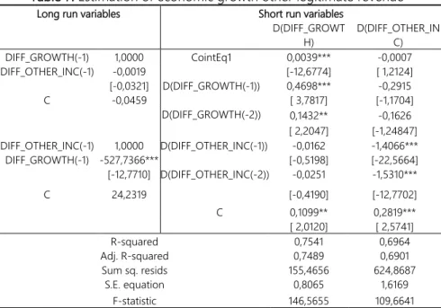
Economic growth and other legitimate revenue. The estimation results in Table 7 show that economic growth with other legitimate revenue in the long run, economic growth has a significant affect on other legitimate revenue at 99% confidence level with a coefficient of -527,7366. In contrary, other legitimate revenue does not have a significant affect on long run economic growth.
The estimation result in the short run, found that each variable only affects itself in the first lag and the second lag. The economic variable does not have a significant affect on other legitimate revenue, likewise other legitimate revenue variables also has not a significant affect on economic growth in the short run. Economic growth has a significant affect on itself in the first lag with a coefficient of 0,4698 at a confidence level of 99% and in the second lag with a coefficient of 0,1432 at a confidence level of 95%. That means, economic growth of 1% in one and two previous periods increased economic growth of 0,4698% and 0,1432% at current period.
Other legitimate revenue also has a significant affect on itself with a 99% confidence level in the first lag and the second lag with coefficients of -
1,4066 and -1,5309. That means, an increase in the other legitimate revenue of 1% of the GRDP in the previous period will reduce the current 1,4066% legitimate revenue from GRDP. Increasing 1% in the other legitimate revenue of GRDB in the previous two periods will reduce 1,5309% of the other legitimate revenue from GRDP at current period.
Table 7. Estimation of economic growth other legitimate revenue
Long run variables Short run variables
D(DIFF_GROWT
H) D(DIFF_OTHER_IN C)
DIFF_GROWTH(-1) 1,0000 CointEq1 0,0039*** -0,0007
DIFF_OTHER_INC(-1) -0,0019 [-12,6774] [ 1,2124]
[-0,0321] D(DIFF_GROWTH(-1)) 0,4698*** -0,2915
C -0,0459 [ 3,7817] [-1,1704]
D(DIFF_GROWTH(-2)) 0,1432** -0,1626 [ 2,2047] [-1,24847]
DIFF_OTHER_INC(-1) 1,0000 D(DIFF_OTHER_INC(-1)) -0,0162 -1,4066***
DIFF_GROWTH(-1) -527,7366*** [-0,5198] [-22,5664]
[-12,7710] D(DIFF_OTHER_INC(-2)) -0,0251 -1,5310***
C 24,2319 [-0,4190] [-12,7702]
C 0,1099** 0,2819***
[ 2,0120] [ 2,5741]
R-squared 0,7541 0,6964
Adj. R-squared 0,7489 0,6901
Sum sq. resids 155,4656 624,8687
S.E. equation 0,8065 1,6169
F-statistic 146,5655 109,6641
Explanation: Number in [ ] is a t-statistic; *** significant at level 1%; ** significant at level 5%; * significant at level 10%.
Source: LHP-LKPD, be treated (BPK 2005-2015)
The value of speed of adjustment coefficient of economic growth equation is 0,0039. This means that the adjustment of economic growth to return to equilibrium is very slow. The coefficient of 0,0039 indicates that the equilibrium adjustment of economic growth in the previous period will be corrected by -0,39% in the current period. Meanwhile, the coefficient of speed of adjustment of other legitimate revenue is not significant.
Based on the estimation results in Table 7, the short run equation model of economic growth and other legitimate revenue are:
∆𝛿𝛿𝑑𝑑𝑑𝑑𝑑𝑑_ 𝑔𝑔𝑡𝑡ℎ𝑟𝑟𝑔𝑔_𝑑𝑑𝑖𝑖𝑖𝑖𝑖𝑖𝑖𝑖= −0,0007 (𝛿𝛿𝑑𝑑𝑑𝑑𝑑𝑑_𝑔𝑔𝑡𝑡ℎ𝑟𝑟𝑔𝑔_𝑑𝑑𝑖𝑖𝑖𝑖 𝑖𝑖𝑖𝑖−1−
527,7365 𝛿𝛿𝑑𝑑𝑑𝑑𝑑𝑑_𝑔𝑔𝑔𝑔𝑔𝑔𝑔𝑔𝑡𝑡ℎ 𝑖𝑖𝑖𝑖−1+ 24,2319)−1,4066 ∆𝛿𝛿𝑑𝑑𝑑𝑑𝑑𝑑_𝑔𝑔𝑡𝑡ℎ𝑟𝑟𝑔𝑔_𝑑𝑑𝑖𝑖𝑖𝑖 𝑖𝑖𝑖𝑖−1 − 1,5309 ∆𝛿𝛿𝑑𝑑𝑑𝑑𝑑𝑑_𝑔𝑔𝑡𝑡ℎ𝑟𝑟𝑔𝑔_𝑑𝑑𝑖𝑖𝑖𝑖 𝑖𝑖𝑖𝑖−2 − 0,2915 ∆𝛿𝛿𝑑𝑑𝑑𝑑𝑑𝑑_𝑔𝑔𝑔𝑔𝑔𝑔𝑔𝑔𝑡𝑡ℎ_𝑑𝑑𝑖𝑖𝑖𝑖 𝑖𝑖𝑖𝑖−1 −
0,1626 ∆𝛿𝛿𝑑𝑑𝑑𝑑𝑑𝑑_𝑔𝑔𝑔𝑔𝑔𝑔𝑔𝑔𝑡𝑡ℎ 𝑖𝑖𝑖𝑖−2+ 0,2819 (13)
∆𝛿𝛿𝑑𝑑𝑑𝑑𝑑𝑑_ 𝑔𝑔𝑔𝑔𝑔𝑔𝑔𝑔𝑡𝑡ℎ𝑖𝑖𝑖𝑖= 0,0039 (𝛿𝛿𝑑𝑑𝑑𝑑𝑑𝑑_𝑔𝑔𝑡𝑡ℎ𝑟𝑟𝑔𝑔_𝑑𝑑𝑖𝑖𝑖𝑖 𝑖𝑖𝑖𝑖−1−
527,7365 𝛿𝛿𝑑𝑑𝑑𝑑𝑑𝑑_𝑔𝑔𝑔𝑔𝑔𝑔𝑔𝑔𝑡𝑡ℎ 𝑖𝑖𝑖𝑖−1+ 24,2319)−0,0161 ∆𝛿𝛿𝑑𝑑𝑑𝑑𝑑𝑑_𝑔𝑔𝑡𝑡ℎ𝑟𝑟𝑔𝑔_𝑑𝑑𝑖𝑖𝑖𝑖 𝑖𝑖𝑖𝑖−1 − 0,0250 ∆𝛿𝛿𝑑𝑑𝑑𝑑𝑑𝑑_𝑔𝑔𝑡𝑡ℎ𝑟𝑟𝑔𝑔_𝑑𝑑𝑖𝑖𝑖𝑖 𝑖𝑖𝑖𝑖−2 + 0,4698 ∆𝛿𝛿𝑑𝑑𝑑𝑑𝑑𝑑_𝑔𝑔𝑔𝑔𝑔𝑔𝑔𝑔𝑡𝑡ℎ_𝑑𝑑𝑖𝑖𝑖𝑖 𝑖𝑖𝑖𝑖−1 +
0,1432 ∆𝛿𝛿𝑑𝑑𝑑𝑑𝑑𝑑_𝑔𝑔𝑔𝑔𝑔𝑔𝑔𝑔𝑡𝑡ℎ 𝑖𝑖𝑖𝑖−2+ 0,1099 (14)
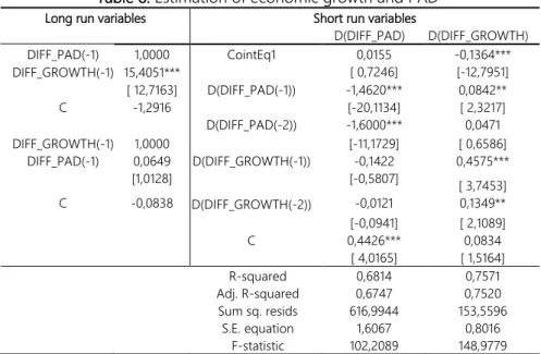
Economic growth and PAD. The estimation results in Table 8 between economic growth and PAD can be found in the long run PAD does not have a significant effect on economic growth. On the other hand, economic growth in the long run has a significant affect on PAD at a 99% confidence level with a coefficient of 15,4051. That is, a 1% increase in economic growth in the long run will affect the increase in PAD of 15,4051% of GRDP.
Economic growth in the first lag and the second lag significantly affects itself at a 99% confidence level in the first lag and 95% in the second lag. In the first lag the coefficient of economic growth is 0,4575 and the second lag is 0,1349. That means, the economic growth in the first lag contributed to the current economic growth of 0,4574% and the second lag contributed 0,1349%.
The coefficient of economic growth is 0.4575 and the second lag is 0,1349. That is, the economic growth in the first lag contributed to the current economic growth of 0,4574% and the second lag contributed 0,1349%. Similarly, significant PAD affects itself at the 99% confidence level with a coefficient of - 1,4619 in the first lag and -1,6000 in the second lag. That is, the PAD in the first lag contributes -1,4619% of the current GRDP to the PAD. The second lag contributes to -1,6000% of current GRDP to PAD.
Table 8. Estimation of economic growth and PAD
Long run variables Short run variables
D(DIFF_PAD) D(DIFF_GROWTH)
DIFF_PAD(-1) 1,0000 CointEq1 0,0155 -0,1364***
DIFF_GROWTH(-1) 15,4051*** [ 0,7246] [-12,7951]
[ 12,7163] D(DIFF_PAD(-1)) -1,4620*** 0,0842**
C -1,2916 [-20,1134] [ 2,3217]
D(DIFF_PAD(-2)) -1,6000*** 0,0471 DIFF_GROWTH(-1)
DIFF_PAD(-1) 1,0000 [-11,1729] [ 0,6586]
0,0649
[1,0128] D(DIFF_GROWTH(-1)) -0,1422
[-0,5807] 0,4575***
[ 3,7453]
C -0,0838 D(DIFF_GROWTH(-2)) -0,0121 0,1349**
[-0,0941] [ 2,1089]
C 0,4426*** 0,0834
[ 4,0165] [ 1,5164]
R-squared 0,6814 0,7571
Adj. R-squared 0,6747 0,7520
Sum sq. resids 616,9944 153,5596
S.E. equation 1,6067 0,8016
F-statistic 102,2089 148,9779 Explanation: Number in [ ] is a t-statistic; *** significant at level 1%; ** significant at level 5%; * significant at level 10%.
Source: LHP-LKPD, be treated (BPK 2005-2015)
The value of speed of adjustment coefficient of economic growth equation is -0,1364. This means that the adjustment of economic growth to return to equilibrium is quite slow. The coefficient of -0,1364 shows that the economic growth equilibrium adjustment in the previous period was corrected
by 13,64% in the current period. Meanwhile, the value of the speed of adjustment PAD coefficient is not significant.
Based on the estimation results in Table 8, the short run equation model of economic growth and PAD are:
∆𝛿𝛿𝑑𝑑𝑑𝑑𝑑𝑑_ 𝑡𝑡𝑔𝑔𝑡𝑡𝑡𝑡𝑡𝑡_ 𝑃𝑃𝑃𝑃𝑃𝑃𝑖𝑖𝑖𝑖= 0,0154 (𝛿𝛿𝑑𝑑𝑑𝑑𝑑𝑑_𝑡𝑡𝑔𝑔𝑡𝑡𝑡𝑡𝑡𝑡_𝑃𝑃𝑃𝑃𝑃𝑃 𝑖𝑖𝑖𝑖−1+
15,4050 𝛿𝛿𝑑𝑑𝑑𝑑𝑑𝑑_𝑔𝑔𝑔𝑔𝑔𝑔𝑔𝑔𝑡𝑡ℎ 𝑖𝑖𝑖𝑖−1−1,2915)−1,4619 ∆𝛿𝛿𝑑𝑑𝑑𝑑𝑑𝑑_𝑡𝑡𝑔𝑔𝑡𝑡𝑡𝑡𝑡𝑡_𝑃𝑃𝑃𝑃𝑃𝑃 𝑖𝑖𝑖𝑖−1 − 1,6000 ∆𝛿𝛿𝑑𝑑𝑑𝑑𝑑𝑑_𝑡𝑡𝑔𝑔𝑡𝑡𝑡𝑡𝑡𝑡_𝑃𝑃𝑃𝑃𝑃𝑃 𝑖𝑖𝑖𝑖−2 − 0,1421 ∆𝛿𝛿𝑑𝑑𝑑𝑑𝑑𝑑_𝑔𝑔𝑔𝑔𝑔𝑔𝑔𝑔𝑡𝑡ℎ 𝑖𝑖𝑖𝑖−1 −
0,0120 ∆𝛿𝛿𝑑𝑑𝑑𝑑𝑑𝑑_𝑔𝑔𝑔𝑔𝑔𝑔𝑔𝑔𝑡𝑡ℎ 𝑖𝑖𝑖𝑖−2+ 0,4426 (15)
∆𝛿𝛿𝑑𝑑𝑑𝑑𝑑𝑑_ 𝑔𝑔𝑔𝑔𝑔𝑔𝑔𝑔𝑡𝑡ℎ𝑖𝑖𝑖𝑖= −0,1364 (𝛿𝛿𝑑𝑑𝑑𝑑𝑑𝑑_𝑡𝑡𝑔𝑔𝑡𝑡𝑡𝑡𝑡𝑡_𝑃𝑃𝑃𝑃𝑃𝑃 𝑖𝑖𝑖𝑖−1+
15,4050 𝛿𝛿𝑑𝑑𝑑𝑑𝑑𝑑_𝑔𝑔𝑔𝑔𝑔𝑔𝑔𝑔𝑡𝑡ℎ 𝑖𝑖𝑖𝑖−1−1,2915) + 0,0841 ∆𝛿𝛿𝑑𝑑𝑑𝑑𝑑𝑑_𝑡𝑡𝑔𝑔𝑡𝑡𝑡𝑡𝑡𝑡_𝑃𝑃𝑃𝑃𝑃𝑃 𝑖𝑖𝑖𝑖−1 + 0,0470 ∆𝛿𝛿𝑑𝑑𝑑𝑑𝑑𝑑_𝑡𝑡𝑔𝑔𝑡𝑡𝑡𝑡𝑡𝑡_𝑃𝑃𝑃𝑃𝑃𝑃 𝑖𝑖𝑖𝑖−2 + 0,4575 ∆𝛿𝛿𝑑𝑑𝑑𝑑𝑑𝑑_𝑔𝑔𝑔𝑔𝑔𝑔𝑔𝑔𝑡𝑡ℎ 𝑖𝑖𝑖𝑖−1 +
0,1349 ∆𝛿𝛿𝑑𝑑𝑑𝑑𝑑𝑑_𝑔𝑔𝑔𝑔𝑔𝑔𝑔𝑔𝑡𝑡ℎ 𝑖𝑖𝑖𝑖−2+ 0,0833 (16)
5. Granger Causality Test with PVECM
Granger Causality Test is conducted to determine the direction of causality between economic growth with tax revenue, economic growth with retribution revenue, economic growth with regional wealth revenue, economic growth with other legitimate revenue, and economic growth with PAD.
Based on the test results in Table 9, it is known that there is a one-way relationship namely tax revenue to economic growth. This is consistent with the PVECM estimates in Table 4. The probability value is 0,0077 <0,05 in the first lag and 0,0171 <0,05 in the second lag, which means that tax revenue has a significant affect on economic growth in the short run.
In the second Granger test between economic growth and retribution revenue, it was found that there was a reciprocal or two-way relationship.
Economic growth affects retribution revenue and retribution revenue affects economic growth. This is consistent with the results of the PVECM estimation in Table 5. The probability value is 0,00 <0,05 in the first lag and 0,00 <0,05 in the second lag, which means that revenue retribution and economic growth have significant affect in the short run.
The third Granger test between economic growth and regional wealth revenue, there is a one-way relationship namely regional wealth revenue to economic growth. This is consistent with the PVECM estimates in Table 6 before.
Probability value 0,0049 <0,05 in the first lag and 0,0001 <0,05 in the second lag, which means that regional wealth revenue has a significant affect on economic growth in the short run.
Table 9. PVECM Granger Causality Test results Endogenous
variables Exogenous variables
∆growth t-2 ∆tax_inc t-2 ∆growth t-1 ∆tax_inc t-1
∆growth -- 8,1333
(0,0171) -- 7,0907
(0,0077)
∆tax_inc 0,9997
(0,6066) -- 0,3417
(0,5588) -- Endogenous
variables Exogenous variables
∆growth t-2 ∆ret_inc t-2 ∆growth t-1 ∆ret_inc t-1
∆growth -- 5,5568
(0,0000) -- 19,7345
(0,0000)
∆ret_inc 2,2075
(0,0000) -- 1,1267
(0,0000) -- Endogenous
variables Exogenous variables
∆growth t-2 ∆rich_inc t-2 ∆growth t-1 ∆rich_inc t-1
∆growth -- 1,9357
(0,0001) -- 7,9275
(0,0049)
∆rich_inc 3,9384
(0,1396) -- 0,7889
(0,3744) -- Endogenous
variables Exogenous variables
∆growth t-2 ∆other_inc t- 2
∆growth t-1 ∆other_inc t- 1
∆growth -- 1,6063
(0,8727) -- 7,9275
(0,6939)
∆other_inc 0,2772
(0,4479) -- 0,7889
(0,9466) -- Endogenous
variables Exogenous variables
∆growth t-2 ∆pad t-2 ∆growth t-1 ∆pad t-1
∆growth -- 8,9042
(0,2964) -- 1,0905
(0,0117)
∆pad 0,8674
(0,6481) -- 0,9116
(0,3397) --
Source: LHP-LKPD, be treated (BPK 2005-2015)
The fourth Granger test between economic growth and other legitimate revenue does not occur in a mutually influential relationship. This is consistent with the PVECM estimates in Table 7. The probability value of the two variables in the first lag and the second lag is greater than 0.05, meaning that other
legitimate revenue and economic growth are not mutually influential in the short run.
The fifth Granger test between economic growth and PAD has a one- way relationship, namely PAD to economic growth. This is consistent with PVECM estimates in Table 8. The probability value is 0,0117 <0,05 in the first lag and 0,2964> 0,05 in the second lag, which means that PAD has a significant affect on economic growth in the short run, especially in the first lag.
The finding of the relationship between the one-way variable tax revenue towards the variable economic growth has a positive and significant direction in line with the research of Easterly and Rebelo (1993), Iimi (2005), Arnold (2008), Hammond and Tosun (2009), Myles (2009), Xing (2011 ), Bacarreza, Vazquez, and Vulovic (2013), Bujang, Hakim, and Ahmad (2013), Stoilova and Patonov (2013), Szarowska (2013), Devkota (2014), Mutiara (2015), Takumah and Iyke (2015) , Saidin, Basit, and Hamza (2016), as well as Stoilova (2017).
The findings of the reciprocal/two-way relationship between the retribution revenue variable and the variable economic growth are positively and significantly directed in line with Mutiara (2015) research. However, Mutiara (2015) only examines the relationship of retribution revenue to economic growth and not vice versa. The findings of the one-way relationship between the PAD variable and the variable economic growth are positively and significantly directed in line with Putri's research (2015), Hedriwiyanto (2016), Rori, Luntungan, and Niode (2016), Manek and Badrudin (2016), Muti'ah (2017) .
6. Test the equation models
The equation models to be tested are equations (8), (9), (10), (12), and (16), which are equations that have significance between independent variables and non-independent variables in the estimation of the PVECM models. Test model equations using stability test, portmanteau normality test, linearity test, heteroscedacity test, and multicollinearity test. The result is that the equation model is free from the assumptions of symptoms of instability with modulus of value below one, free from abnormalities, linear functioning equations, free from heteroscedacity and multicolinearity occurring only in long run economic growth variables.
7. Summary of findings of PVECM estimation and Granger Causality Test After the classic assumption test, it can be said that the equation models obtained from the PVECM estimation is the best equation models. Therefore, the results of the PVECM estimation can be summarized to more easily understand the findings in this study shown in Table 10.