It is found that the velocity of the solitary wave of the electromagnetic vector depends on the amplitude of all components of the field in a linear manner. The frequency spectra of the single waves are calculated and their low-frequency content is highlighted. 213-2141, is the union between different components of the same vector field, which creates the interaction between these components.
S t is precisely this type of plasma that is commonly encountered in astrophysics and ionospheric physics. To rewrite this integral in terms of the electric field, we use Maxwell's equation (2.4) in the space G. In particular, the main efforts are focused on the study of stationary wave solutions.
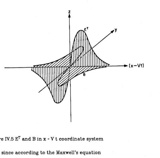
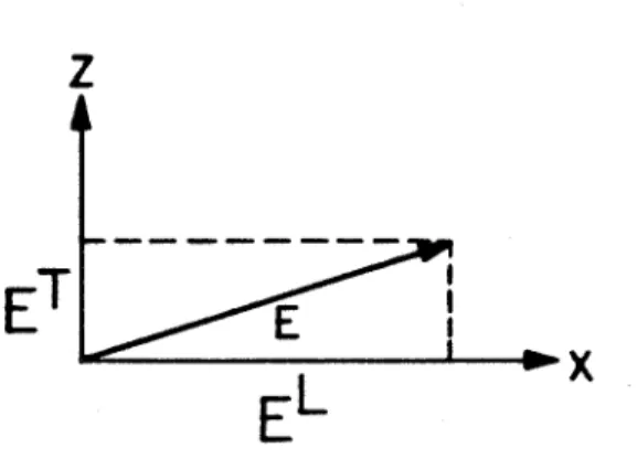
Let x also denote the direction of propagation, and z the direction of the transverse component of the electric field (see Figure 1). The new potentials u and v correspond to the longitudinal and transverse components of the E field, respectively, and have a velocity dimension. In this paragraph we will study the local distribution of electrons in a certain band A x (see Fig. 111-3.).
The right-hand side of the third equation in (3.31) has a resonant term (proportional to sense 6), which gives rise to a secular term in the solution.
Interacting Solitary Waves
The solution of (2.51) can be easily obtained if we seek it in a form F = Aflfz, where A is a constant. The next equation in the hierarchy has zero on the right-hand side, so F can be approximated by . Equation (3.54) approximates a single wave with a , for regions where f l a 1 and f 2 is either large or small, and for regions where f 2 fil 1 and f , is either large or small, describes a wave alone with
Whitham (1977) developed a numerical method for the KdV equation with a periodic initial value problem that allows solitary wave interaction to be investigated. Although we have obtained the qualitative characteristics of the soliton interaction governed by (3.41), further numerical verification of the interaction is required. It is shown that solutions of the initial value problem for this equation have better smoothness properties than those for the KdV equation.
In the preceding analysis, we will adopt Benjamin's approach to stability analysis for the KdV equation to show that the solitons governed by (3.59) are also stable. The solitary wave solution ii will be compared to a class of solutions u(x,t) that evolve from some initial conditions that are in some sense close to those for Ti. Intuitively, the stability of Ti can be seen as if a t t = 0, ii and u are close to each other.
The result in the form of (3.60) not only implies uniform temporal boundedness of the variance of the difference A = u -a and its x derivative, but from the point of view of (A-2) (see Appendix A), (3.60 ) implies that the magnitude of A is uniformly bounded everywhere . To determine the stability of a solitary wave solution. 3.59) we need to find two nonlinear functionals that are invariant with time for solutions (3.59). The functionals N(u) and M(u) will play a key role in determining the stability of the solitary wave solution (3.59).
To obtain a lower bound for 6N, we first note that a is an even function (3.69) which can be rewritten as This is the required result according to system (3.61). Using the right-hand side of (3.79) and (3.70), we can determine D as the positive root of the following equation. We want to show that the Cm solutions of (3.6), which together with their x derivatives tend to zero as x -, k m , are uniquely determined by their initial values.
Conservation Laws and Lagrangian
Conservation law (3.95) follows directly from (3.59) simply by grouping the appropriate terms, and identity (3.96) can be obtained by multiplying (3.59) by 2u and rearranging the appropriate terms. Scott et al, [1973] show that if the equation under consideration can be derived from Lagrangian density, which does not explicitly depend on time, then this equation can be considered lossless, or conservative in the conventional sense. In the other paper, Whitham [1974] uses various manipulations of the mean Lagrangian density in the study of slowly varying wave trains.
Note that while most of the evolution equations known to us, including the KdV and Boussinesq equations, are invariant under the Galilean transformation. Formula (4.6) shows the dependence of the eigenvalue hl on the amplitude a of the longitudinal wave u, which again shows the connection between the two components EL and ET. The constant in (4.9) can be determined from the initial conditions, so the energy of some initial pulses will be split into energies carried by longitudinal and transverse waves.
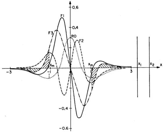
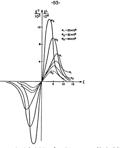
It is convenient, for computational purposes, to express all hypergeometric functions in (4.32) and (4.33) in the form that can be easily executed on a computer. Due to the complex nature of the hypergeometric functions, it is difficult to see the graphical representation of the solution (4.33). However, using the relationships we can numerically evaluate ET, for different values of hl and r2.
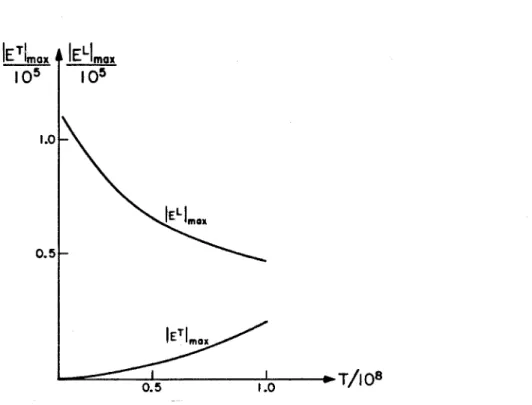
It can be explained, perhaps, due to the rapid convergence of the hypergeometric series in the region 0 < X < m (0 < z < k), and the relatively slow rate of convergence of the same series in the region - = < X < 0. It is observed that increasing the number of terms in the series enlarges the tail (negative part) of ET, but keeping the waveform of ET almost unchanged. Although not shown here, numerical results show that an increase in a produces a shift in both I E:, I and ]EL I curves upward, while a decrease in a.
We will look for solitary wave solutions for longitudinal and transverse waves, u and v. Note that we have assumed a new wave speed V instead of U defined in (3.7), since it is reasonable to assume that the speed of a two-component wave (EL and ET) should generally be different from the speed of a longitu - dinal wave, but the former should reduce to of the other in the limit when. We thought that these adjustments were not necessary in the case where the waves were predominantly longitudinal.
This allows us to solve (4.50) and then match its solution with the solution obtained by solving (4.52), if the latter is possible. By examining (4.55) we immediately see that when the transverse component of the wave is zero, the parenthetical expression is zero, which requires b l + m so that v would vanish.
Generalization of the Wave Velocity
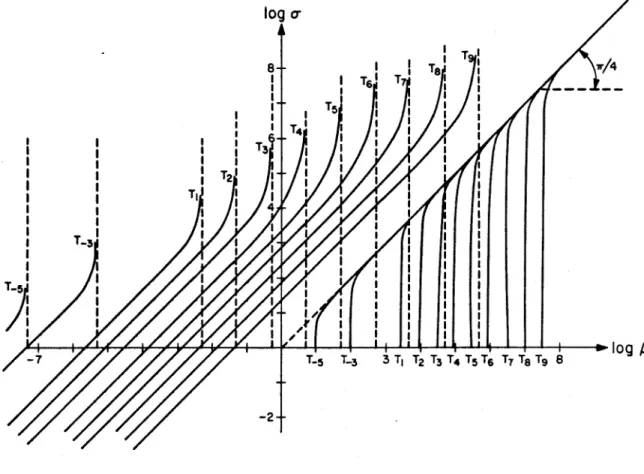
Numerous computer runs were made to determine the values of a t h a t would support a given @, for different temperatures, numerically. In most regions of interest a depends on @ improperly, and for any temperature Tn = l o n , n is real, there is a region, t h a t can be approximated by the following inequalities. Thus, the velocity V of the two-component wave also depends linearly on the amplitude of the transverse component.
S D m PKYSICALKEMARKS
Motion of the Electron in a Solitary Field
Consequently, electron in the longitudinal direction also undergoes finite dissipation which is given by (5.25). Although the amplitude of the longitudinal wave does not appear in (5.27), it does contribute to the energy density since @, must be supported by longitudinal component a,. The velocity of a vector solitary electromagnetic wave depends linearly on the amplitude of each component of the field.
Moreover, the relationship between the amplitudes of the longitudinal and transverse waves is likewise linear for physically reasonable ranges of amplitude and plasma temperature. While the increase in plasma temperature tends to reduce the amplitude and to broaden the longitudinal wave profile, it leads to larger amplitudes of the transverse waves in the case where the waves are predominantly longitudinal. The longitudinal solitary waves are stable in the Lyapunov sense, and the analysis of a periodic wave train solution indicates that the equation for these waves is hyperbolic in nature.
The longitudinal wave equation can be derived from a Lagrangian density function; accordingly, the wave equation is 'lossless', or conservative in the conventional sense. Although the qualitative features of the soliton interaction are obtained, further numerical verification of the interaction is needed. We assume that for all t , the solution u is, as a function of x, an element of the Sobler function space W$(R).
The estimation of the lower bounds for 6"(r) as well as b2N(s) will be based on the spectral theory of singular boundary value problems. In order to have b2N(r) r J, we want the negative part to be the integrand in (C.2) larger than the negative part the integrand in (C.3) compared to the terms in r$ in (C.2) and (C.3), respectively.We wish to expand the expression sech2y as a linear combination of eigenfunctions of the associated eigenvalue problem.
In our case, eigenvalue spectrum consists of a finite number of discrete negative values, together with a continuous spectrum on the interval [0, m). The only value of Q in (C.5) that enables us to express the sech2y as a linear combination of the eigenvalues of the problem (C.5) is 20. This coefficient also ensures the negative part of the integrand in (C. 2) be greater than the corresponding term in (c.3), compared to r'2 terms.
To further reduce (C.14) we first note that sech2y can be expressed as a linear combination of the eigenfunctions q l and q2, namely. Exact N-soliton solutions of the wave equation of long waves in shallow water and nonlinear lattices.