CHAPTER IV
FINDINGS AND DISCUSSION
In this chapter writer explain about the result of the study discussion A. The Presentation of Data
In this section, it would be describe the obtained data of improvement students’ vocabulary after and before taught by using advertisement. The present data consists of distribution of pre-test score of pre experiment class.
1. Distribution of pre-test of pre experiment class
The pre-test of the pre experiment class is present in the following table
Table 4.1
Score of pre-test of the data achieved by the students
No Name Score
1. R01 61.4
2. R02 45.7
3. R03 47.1
4. R04 37.1
5. R05 28.6
6. R06 62.8
7. R07 45.7
8. R08 68.5
9. R09 62.8
10. R10 60
11. R11 48.6
12. R12 57.1
13. R13 40
14. R14 62.8
15. R15 27.1
16. R16 64.2
17. R17 50
18. R18 65.7
19. R19 50
20. R20 57.1
21. R21 55.8
22. R22 58.5
23. R23 37.1
24. R24 28.6
25. R25 48.6
26. R26 42.8
27. R27 61.4
28. R28 65.7
29. R29 68.5
30. R30 50
Table above describe the score of each student and show the student who passed and failed the test. It shows, there are 11 students who passed the test or about 36.67 % in percentage and there are 19 students who failed the test or about 63.33 % in percentage.
Based on the data above, it can be see that the student’s highest score is 68.5 and the student’s lowest score is 27.1. However, based on the evaluation standard of English subject, there are 19 students who failed, they get fewer than 60.
Table 4.2
The Frequency Distribution of Pre-test score No Score (X) Frequency
( f )
Fx
1. 68.5 2 137
2. 65.7 2 131.4
3. 64.2 1 64.2
4. 62.8 3 188.4
5. 61.4 2 122.8
6. 60 1 60
7. 58.5 1 58.5
8. 57.1 2 114.2
9. 55.8 1 55.8
10. 50 3 150
11. 48.6 2 97.2
12. 47.1 1 47.1
13. 45.7 2 91.4
14. 42.8 1 42.8
15. 40 1 40
16. 37.1 2 74.2
17. 28.6 2 57.2
18. 27.1 1 27.1
TOTAL 𝑓 =30 𝑓𝑥=1.559.3
The distribution of students’ pre-test score can also be see in the following figure :
Figure 4.1
Histogram of Frequency Distribution of Pre-test
The table and figure above show the students’ pre-test score of the pre experiment class. It could be see that there is 1 student get score 27.1. There are 2 students get score 28.6. There are 2 students get score 37.1. There is 1 student get score 40. There is 1 student get score 42.8. There are 3 students get score 50. There is 1 student get score 55.8. There are 2 students get score 57.1. There is 1 student get score 58.8. There is 1 student get score 60. There are 3 students get score 62.8. There is 1 student get score 64.2. There are 2 students get score 65.7. There are 2 students get score 68.5. In this case, many students get score under 60.
0 1 2 3
68.5 65.7 64.2 62.8 61.4 60 58.5 57.1 55.8 50 48.6 47.1 45.7 42.8 40 37.1 28.6 27.1
The Frequency Distribution of Pretest score
Frequensi
Table 4.3
The Calculation of Mean of Pre-Test Score
The next step, the writer tabulated the score into the table for calculation mean as follows:
No Score (X) Frequency ( f )
Fx Fkb Fka
1. 68.5 2 137 30 1
2. 65.7 2 131.4 28 3
3. 64.2 1 64.2 27 5
4. 62.8 3 188.4 24 6
5. 61.4 2 122.8 22 9
6. 60 1 60 21 11
7. 58.5 1 58.5 20 12
8. 57.1 2 114.2 18 13
9. 55.8 1 55.8 17 15
10. 50 3 150 14 16
11. 48.6 2 97.2 12 19
12. 47.1 1 47.1 11 21
13. 45.7 2 91.4 9 22
14. 42.8 1 42.8 8 24
15. 40 1 40 7 25
16. 37.1 2 74.2 5 26
17. 28.6 2 57.2 3 28
18. 27.1 1 27.1 2 30
TOTAL 𝑓 =30 𝑓𝑥=1.559.3
From the table above, the data could be interest in the formula of mean. In simple explanation, X is score of students, f is total students who get the score, Fx is multiplication both X and f, Fkb is the comulative students calculate from under to the top, in other Fka is the comulative students calculate from the top to under.
a. Mean M = 𝑓𝑥𝑁
M = 1.559.330 M = 51.97667 M = 51.97
The calculation above shows of mean value is 51.9
The last step, the writer tabulated the scores of pre-test of Pre experimental class into the table for the calculation of standard deviation and the standard error as follows
Table 4.4
The Calculation of the Standard Deviation and Standard Error of the Pre-test Score
No Score (X) Frequency ( f )
Fx X 𝑿𝟐 𝒇𝒙𝟐
1. 68.5 2 137 16.6 275.56 551.12
2. 65.7 2 131.4 13.8 190.44 380.88
3. 64.2 1 64.2 12.3 151.29 151.29
4. 62.8 3 188.4 10.9 118.81 356.43
5. 61.4 2 122.8 9.5 90.25 180.5
6. 60 1 60 8.1 65.61 65.51
7. 58.5 1 58.5 6.6 43.56 43.56
8. 57.1 2 114.2 5.2 27.04 27.04
9. 55.8 1 55.8 3.9 15.21 15.21
10. 50 3 150 -1.9 3.61 10.83
11. 48.6 2 97.2 -3.3 10.89 21.78
12. 47.1 1 47.1 -4.8 23.04 23.04
13. 45.7 2 91.4 -6.2 38.44 76.88
14. 42.8 1 42.8 -9.1 82.81 82.81
15. 40 1 40 -11.9 141.61 141.61
16. 37.1 2 74.2 -14.8 219.04 438.08
17. 28.6 2 57.2 -23.3 542.89 1,085.78
18. 27.1 1 27.1 24.8 615.04 615.04
TOTAL 𝑓 =30 𝑓𝑥=1.55 2𝑓𝑥 =
9.3 4294.53
The table above used for calculate standard deviation and standard error by calculate standard deviation first. The process of calculation uses formula below:
a. Standard Deviation SD = 𝑓𝑥2
𝑁
SD = 4294.5330 SD = 143.151
SD =11.9645727044470752 SD = 12.1
b. Standard Error 𝑆𝐸𝑀𝐷 = 𝑆𝐷𝐷
𝑁−1
𝑆𝐸𝑀𝐷 = 11.9645727044470752 30−1
𝑆𝐸𝑀𝐷 = 11.9645727044470752 29
𝑆𝐸𝑀𝐷 = 11.9645727044470752 5.38516480713
𝑆𝐸𝑀𝐷 = 2.2217
The result of calculation shows the standard deviation of pre-test score is 12.1 and the standard error of pre-test is 2.2217.
The writer also calculated the data calculation of pre-test score of pre- experiment class using SPSS 18.0 program. The result statistic table as follows:
Table 4.5
The Frequency Distribution of Pre-test Score using SPSS 18.0 Program Statistics
Pretest
N Valid 30
Missing 0
Pretest
Frequency Percent
Valid Percent
Cumulative Percent
Valid 27.1 1 3.3 3.3 3.3
28.6 2 6.7 6.7 10.0
37.1 2 6.7 6.7 16.7
40.0 1 3.3 3.3 20.0
42.8 1 3.3 3.3 23.3
45.7 2 6.7 6.7 30.0
47.1 1 3.3 3.3 33.3
48.6 2 6.7 6.7 40.0
50.0 3 10.0 10.0 50.0
55.8 1 3.3 3.3 53.3
57.1 2 6.7 6.7 60.0
58.5 1 3.3 3.3 63.3
60.0 1 3.3 3.3 66.7
61.4 2 6.7 6.7 73.3
62.8 3 10.0 10.0 83.3
64.2 1 3.3 3.3 86.7
65.7 2 6.7 6.7 93.3
68.5 2 6.7 6.7 100.0
Total 30 100.0 100.0
The table above shows the result of pre-test scores achieved by the experiment class using SPSS 18.0 program. It could be see there is 1 student who get score 27.1 (3.3%). There are two students who get score 28.6 (6.7%). There are 2 students who get score 37.1 (6.7%). There is 1 student who get score 40 (3.3%).There is 1 student who get score 42.8 (3.3%). There are 2 students who get score 45.7 (6.7%).There is 1 student who get score 47.1 (3.3%) .There are 2 students who get score 48.6 (6.7%).There are 3 students who get score 50 (10.0%) There is 1 student who get
score 58.5 (3.3%). And there is 1 student who get score 60 (3.3%).There are 2 students who get score 61.4 (6.7%).There are 2 students who get score 62.8 (10.0%).There is 1 student who get score 64.2 (3.3%).There are 2 students who get score 65.7 (6.7%). And there are 2 students who get score 68.5 (6.7%).
The next step, the writer calculated the scores of mean, standard deviation of mean of pre-test in experiment class using SPSS as follows:
Table 4.6
The Table of Calculation of Mean, and Standard Deviation of Mean of Pre-test Scores Using SPSS 18.0 Program
Descriptive Statistics
N Minimum Maximum Mean
Std.
Deviation
Pretest 30 27.1 68.5 51.977 12.1689
Valid N
(listwise)
30
The table shows the result of mean calculation was 51.9. The result of standard deviation is 12.1
2. Distribution of post-test of pre experiment class
The post-test of the pre experiment class is present in the following table Table 4.7
Score of post-test of the data achieved by the students
No Name Score
1. R01 80
2. R02 74.2
3. R03 74.2
4. R04 68.5
5. R05 72.8
6. R06 77.1
7. R07 75.7
8. R08 78.5
9. R09 77.1
10. R10 77.1
11. R11 64.2
12. R12 78.5
13. R13 78.5
14. R14 70
15. R15 77.1
16. R16 85.7
17. R17 64.2
18. R18 74.2
19. R19 74.2
20. R20 82.8
21. R21 71.4
22. R22 88.5
23. R23 74.2
24. R24 87.1
25. R25 68.5
26. R26 77.1
27. R27 77.1
28. R28 72.8
29. R29 80
30. R30 77.1
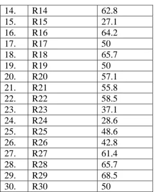
Table above describe the score of each students and show the student who passed and failed in the test. It shows, all of students who passed the test or about 100% in percentage.
Based on the data above, it can be see that student’s highest score is 88.5 and the student’s lowest score is 64.2.However, based on evaluation standard of English subject, no one students who failed , they get fewer than 60.
Table 4.8
The Frequency Distribution of the Post-test
The distribution of student’s post-test score can also be see in the following figure.
No Score (X) Frequency ( f )
Fx
1. 88.5 1 88.5
2. 87.1 1 87.1
3. 85.7 1 85.7
4. 82.8 1 82.5
5. 80 2 160
6. 78.5 3 235.5
7. 77.1 7 539.7
8. 75.7 1 75.7
9. 74.2 5 371
10. 72.8 2 145.6
11. 71.4 1 71.4
12. 70 1 70
13. 68.5 2 137
14. 64.2 2 128.4
TOTAL 𝑓 = 30 𝑓𝑥
= 2278.41
Figure 4.2
Histogram of Frequency Distribution of Post-test Score
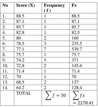
The table and figure above show the students’ post-test score. It could be see that there are 2 students who get score 64.2. There are 2 students who got score 68.5.
There is 1 students who get score 72.8. There is 1 student who get score 71.4. There are 2 students who get score 72.8. And there are 5 students who get score 74.2.There is 1 student who get score 75.7. There are 7 students who get score 77.1. There are 3 students who get score 78.5. There are 2 students who get score 80. There is 1 student who get score 82.8.There is 1 student who get score 85.7. There is 1 student who get score 87.1 and There is 1 student who get score 88.5.
The next step, the writer tabulated the score into the table for the calculation mean as follows:
Table 4.9
0 1 2 3 4 5 6 7 8
88.587.185.782.8 80 78.577.175.774.272.871.4 70 68.564.2
The Frecuency distribution of Post- test score
Frecuency
The Calculation of Mean of Post-test score
The next step, the writer tabulated the score into the table for the calculation mean as follows:
No Score (X) Frequency ( f )
Fx Fkb Fka
1. 88.5 1 88.5 30 2
2. 87.1 1 87.1 29 3
3. 85.7 1 85.7 28 4
4. 82.8 1 82.5 27 5
5. 80 2 160 25 6
6. 78.5 3 235.5 22 8
7. 77.1 7 539.7 15 11
8. 75.7 1 75.7 14 18
9. 74.2 5 371 9 19
10. 72.8 2 145.6 7 24
11. 71.4 1 71.4 6 26
12. 70 1 70 5 27
13. 68.5 2 137 3 28
14. 64.2 2 128.4 1 30
TOTAL 𝑓 = 30 𝑓𝑥
= 2278.41
From the table above, the data could be inserted in the formula of mean. In simple explanation, X is score of students, f is total students who get the score, Fx is multiplication both X and f, fkb is the comulative students calculate from under to the top, in other side fka is the comulative students calculate from the top to under. The process of calculation used formula below.
a. Mean M = 𝑓𝑥𝑁
M= 2278.41
30
M = 75.947 M = 75.94
The calculation above show of mean value is 75.9
The last step, the writer tabulated the score of post-test into the table for the calculation of standard deviation and standard error as follows:
Table 4.10
The Calculation of the Standard Deviation and Standard Error of Post-test
No Score (X) Frequency ( f )
Fx X 𝑿𝟐 𝒇𝒙𝟐
1. 88.5 1 88.5 12.6 158.76 158.76
2. 87.1 1 87.1 11.2 125.44 125.44
3. 85.7 1 85.7 9.8 96.04 96.04
4. 82.8 1 82.5 6.9 47.61 47.61
5. 80 2 160 4.1 16.81 33.63
6. 78.5 3 235.5 2.6 6.76 20.28
7. 77.1 7 539.7 1.2 1.44 10.08
8. 75.7 1 75.7 -0.2 0.04 0.04
9. 74.2 5 371 -1.7 2.89 14.45
10. 72.8 2 145.6 -3.1 9.61 19.22
11. 71.4 1 71.4 -4.5 20.25 20.25
12. 70 1 70 -5.9 34.81 34.81
13. 68.5 2 137 -7.4 54.76 109.52
14. 64.2 2 128.4 -11.7 136.89 273.78
TOTAL 𝑓 = 30 𝑓𝑥
= 2278.41
2𝑓𝑥 =963.9
The table above used for calculate standard deviation and standard error by calculate standard deviation first. The process of calculation use formula below:
a. Standard Deviation SD = 𝑓𝑥2
𝑁
SD = 963.9
30
SD = 32.13
SD = 5.666833308883073553 SD = 5.76
b. Standard Error 𝑆𝐸𝑀𝐷 = 𝑆𝐷𝐷
𝑁−1
𝑆𝐸𝑀𝐷 = 5.6666833308883073553 29
𝑆𝐸𝑀𝐷 = 5.666833308883073553 5.385164807134504
𝑆𝐸𝑀𝐷 = 1.052304527 𝑆𝐸𝑀𝐷 = 1.052
The result of calculation show the standard deviation of post-test is 5.76 and the standard error of post-test score is 1.052.
Table 4.11
The Frequency Distribution of Post-test Scores Using SPSS 18.0 Program
Statistics
Pretest Posttest
N Valid 30 30
Missing 0 0
Posttest
Frequency Percent
Valid Percent
Cumulative Percent
Valid 64.2 2 6.7 6.7 6.7
68.5 2 6.7 6.7 13.3
70.0 1 3.3 3.3 16.7
71.4 1 3.3 3.3 20.0
72.8 2 6.7 6.7 26.7
74.2 5 16.7 16.7 43.3
75.7 1 3.3 3.3 46.7
77.1 7 23.3 23.3 70.0
78.5 3 10.0 10.0 80.0
80.0 2 6.7 6.7 86.7
82.8 1 3.3 3.3 90.0
85.7 1 3.3 3.3 93.3
87.1 1 3.3 3.3 96.7
88.5 1 3.3 3.3 100.0
Total 30 100.0 100.0
The table above shows the result of post-test scores achieved by the experiment class using SPSS 18.0 program. It could be see there are 2 students who get score 64.2 (6.7%). There are 2 students who get score 68.5 (6.7%). There is 1 student who get score 70 (3.3%). There is 1 student who get score 71.4 (3.3%) There are 2 students who get score 72.8 (6.7%). There are 5 students who get score 74.2 (16.7). There is 1 student who get score 75.7 (3.3%). There are 7 students who get score 77.1 (23.3%). There are 2 students who get score 78.5 (6.7%). There are 2 students who get score 80 (6.7%). There is 1 student who get score 82.8 (3.3%).
There is 1 student who get score 85.7 (3.3%). There is 1 student who get score 87.1 (3.3%). And there is 1 student who get 88.5 (3.3%).
The next step, the writer calculated the scores of mean, standard deviation of mean of post-test using SPSS as follows.
Table 4.12
The Table of Calculation of Mean, Standard Deviation, and Standard Error of Mean of Post-test Scores Using SPSS 18.0 Program
Descriptive Statistics
N Minimum Maximum Mean
Std.
Deviation
Posttest 30 64.2 88.5 75.947 5.7650
Valid N
(listwise)
30
The table shows the result of mean calculation is 75.94. The result of standard deviation is 5.76
Table 4.13
The Table of Different score pre and post test
No Pre test Score Post test Score Description of Score
1. 61.4 80 Increased
2. 45.7 74.2 Increased
3. 47.1 74.2 Increased
4. 37.1 68.5 Increased
5. 28.6 72.8 Increased
6. 62.8 77.1 Increased
7. 45.7 75.7 Increased
8. 68.5 78.5 Increased
9. 62.8 77.1 Increased
10. 60 77.1 Increased
11. 48.6 64.2 Increased
12. 57.1 78.5 Increased
13. 40 78.5 Increased
14. 62.8 70 Increased
15. 27.1 77.1 Increased
16. 64.2 85.7 Increased
17. 50 64.2 Increased
18. 65.7 74.2 Increased
19. 50 74.2 Increased
20. 57.1 82.8 Increased
21. 55.8 71.4 Increased
22. 58.5 88.5 Increased
23. 37.1 74.2 Increased
24. 28.6 87.1 Increased
25. 48.6 68.5 Increased
26. 42.8 77.1 Increased
27. 61.4 77.1 Increased
28. 65.7 72.8 Increased
29. 68.5 80 Increased
30. 50 77.1 Increased
Increase in value experienced by all students in grade VII-b, it can be seen post test score higher than pre test score, minimum score of pre-test was 27.1, minimum score of post-test was 64.2, maximum score of pre-test was 68.5 and maximum score of post-test was 88.5.
Table 4.14
The Table of Different Calculation of Mean, Standard Deviation, and Standard Error of Mean between Pre-test and Post-test Scores
No N Minimum Maximum Mean Std.
Deviation
Std.
Error
Pre-test 30 27.1 68.5 51.977 12.1 2.2217
Post-test 30 64.2 88.5 75.947 5.7650 1.052
B. Testing Normality and Homogeneity
Definition of Homogeneity of Variance is when all the variables in statistic data have the same finite or limited variance. When homogeneity of variance is equal for a statistical model. A simple computation approach to analysis the data can be
used due to a low level of uncertainty in the data.1 This equality is homogeneity or homoscedasticity.
1. Testing Normality
Table 4.15 Tests of Normality
Kolmogorov-Smirnova Shapiro-Wilk
Statistic Df Sig. Statistic Df Sig.
Pretest .130 30 .200* .931 30 .053
a. Lilliefors Significance Correction
*. This is a lower bound of the true significance.
a. Test distribution is Normal.
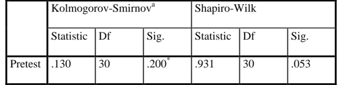
The criteria of the normality test pre-test and post-test is if the value of (probability value/critical value) is higher than or equal to the level of significance alpha defined (r = a), it means that, the distribution is normal.
Based on the calculation using SPSS 18.0 above, the value of r (probably value/critical value) from pre-test and post-test of the experiment class in Kolmogorov-Smirnov table is higher than level of significance alpha used or r
= 0.053> 0.05 (Pre-test) and r = 0.200 > 0.05 (Post-test) so that the distributions are normal. It meant that the students’ score of in pre-test and post-test had a normal distribution.
1AgusIrianto, Statistik:KonsepDasardanAplikasinya, Jakarta: Prenada Media, 2004, p.62.
2. Testing Homogeneity
Table 4.16
Test of Homogeneity of Variances
Levene
Statistic df1 df2 Sig.
1.983 6 16 .128
Table 4.16 ANOVA
Sum of
Squares Df
Mean
Square F Sig.
Between Groups
1573.282 13 121.022 .712 .729
Within Groups 2721.072 16 170.067
Total 4294.354 29
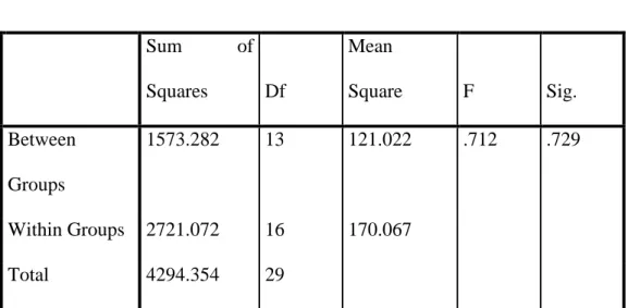
The criteria of the homogeneity test pre-test and post-test was if the value of (probability value/critical value) is higher than or equal to the level of significance alpha defined (r = a), it means that, the distribution is homogeneity. Based on the
calculation using SPSS 18.0 above, the value of (probably value/critical value) from pre-test and post-test of the experiment class on Homogeneity of Variances in sig column is known that p-value was 0.128. The data in this study fulfilled homogeneity since the p value is higher 0.128 > 0.05.
C. Testing Hypothesis using 𝑻𝒕𝒆𝒔𝒕
The writer chose the significance level on 5%, it means the significance level of refusal of null hypothesis on 5%. The writer decided the significance level at 5%
due to the hypothesis type stated on non-directional (two-tailed test). It means that the hypothesis can’t direct the prediction of alternative Hypothesis. Alternative Hypothesis symbolized by “1”. This symbol could direct the answer of hypothesis,
“1” can be (>) or (<). The answer of hypothesis could not be predicted whether on more than or less than.
To test the hypothesis of the study, the writer used t-test statistical calculation.
Firstly, the writer calculated the standard deviation and the error of X1 and X2 at the previous data presentation. In could be seen on this following table:
Table 4.17
The Standard Deviation and Standard Error of X1 and X2
Variable The Standard
Deviation
The Standard Error
X1 12.1689 2.2217
X2 5.7650 1.0525
X1 = Score of pre-test X2 = Score of Post-test
The table shows the result of the standard deviation calculation of X1 is 12.1689and the result of the standard error mean calculation is 2.2217. The result of the standard deviation calculation of X2 is5.7650 and the result of the standard error mean calculation is1.0525.
The next step, the writer calculated the standard error of the differences mean between X1 and X2 as follows:
Standard error of mean of score difference between Variable I and Variable II SEM1 – SEM2 = SEM12
+ SEM22
SEM1 – SEM2 = 2.2217 + 1.0525 2 SEM1 – SEM2 = 4.93595089 + 1.10775625 SEM1 – SEM2 = 6.04370714
SEM1 – SEM2 = 2.4583952367347281 SEM1 – SEM2 = 2.458
The calculation above shows the standard error of the differences mean between X1 and X2 is 2.458. Then, it was inserted to thetoformula to get the value of t observed as follows:
to= 𝑀𝐷 ∕ 𝑆𝐸𝑀𝐷
to= 75.947−51.977 2.458
to= 23.972.458
to= 9.75183
to= 9.751
Which the criteria:
If t-test (t-observed) ≥ t-table, Ha is accepted and Ho is rejected If t-test (t-observed) < t-table, Ha is rejected and Ho is accepted
Then, the writer interpreted the result of t-test; previously, the writer accounted the degree of freedom (df) with the formula:
Df = N -1
= 30 – 1 = 29
5% to 1%
2.04 <9.751> 2.76
The writer chose the significant levels at 5%, it means the significant level of refusal of null hypothesis at 5%. The writer decided the significance level at 5% due to the hypothesis. It meant that the hypothesis can’t direct the prediction of alternative hypothesis. Alternative hypothesis symbolized by “1”. This symbol could direct the answer of hypothesis, “1” can be (>) or (<). The answer of hypothesis could not be predicted whether on more than or less than.
The calculation above shows the result of t-test calculation as in the table follows:
Variable T
observed
T table Df/db
5% 1%
X1-X2 9.751 2.04 2.76 29
Where:
X1 = Score of pre-test X2 = Score of post-test
T observe = the calculated Value T table = the distribution of t value Df/db = Degree of freedom
Based on the result of hypothesis test calculation, it is find that the value of tobserved is greater than the value of table at 1% and 5% significance level or 2.04<9.751
>2.76. It means Ha is accepted and Hois rejected.
It is interpreted based on the result of calculation that Ha stating that the students taught vocabulary by advertisement vocabulary size is accepted. It means that taught by advertisement have given effect in teaching vocabulary size at the seventh students of MTs An-NurPalangka Raya.
D. Testing Hypothesis using SPSS 18.0 ( One Sample T test )
The Standard Deviation and the Standard Error of X using SPSS 18.0.
Table 4.18
The Standard Deviation and the Standard Error of X1 and X2 using SPSS 18.0 Group Statistics
One-Sample Statistics
N Mean
Std.
Deviation
Std. Error Mean
Pretest 30 51.977 12.1689 2.2217
One-Sample Statistics
N Mean
Std.
Deviation
Std. Error Mean
Pretest 30 51.977 12.1689 2.2217 Posttest 30 75.947 5.7650 1.0525
Table 4.19
The Calculation of T-test Using SPSS 18.0 One-Sample Test
Test Value = 0
T Df
Sig. (2- tailed)
Mean Difference
95% Confidence Interval of the Difference
Lower Upper
prestest 23.395 29 .000 51.9767 47.433 56.521
posttest 72.155 29 .000 75.9467 73.794 78.099
The table shows the result of t-test calculation using SPSS 18.0 program.
Since the result of pre test and post-test had difference score of variance, it meant the t-test calculation used at the equal variances not assumed. It found that the result of
𝑡𝑜𝑏𝑠𝑒𝑟𝑣𝑒𝑑are 23.395 and 72.155, the result of mean difference 51.9767 and 75.9467 and the standard error difference are 2.2217 and 1.0525.
E. Interpretation
To examine the truth or the false of null hypothesis stating that the students taught advertisement have better vocabulary size, the result of t-test is interpreted on the result of degree of freedom to get the table. The result of degree of freedom (df) is29, it find from total number of the students in both class minus 1. The following table is the result of tobservedand table from 29df at 5% and 1% significance level.
Table 4.20
The Result of T-test Using SPSS 18.0
The interpretation of the result of t-test using SPSS 18.0 program, it was foundthe 𝑡𝑜𝑏𝑠𝑒𝑟𝑣𝑒𝑑 is greater than the t table at 1% and 5% significance level or 2.04<9.751>2.76. It means that Ha is accepted and Hois rejected.
It could be interpreted based on the result of calculation that Ha stating that the students taught vocabulary by advertisement vocabulary size is accepted. It means
Variable T observed T table Df/db
5% 1%
X1-X2 9.751 2.04 2.76 29
that taught by advertisement have given effect in teaching vocabulary size at the seventh students of MTs An-NurPalangka Raya.
F. Discussion
The result of data analysis shows that the students taught by advertisement give effect to increase vocabulary at the seventh year students of MTs An-Nur ofPalangka Raya. It can be seen first from the means score between Pre-test and Post- test. The mean score of Post-test reached higher score than the mean score of Pre-test (X=51.977< Y=75.94). It indicated that the students’ score increase after conducting treatment. In other words, the students taught by advertisement given effect to increase vocabulary size at the seventh year students of MTs An-NurPalangka Raya”.
Meanwhile, after the data was calculated using the ttest formula using manual calculation shows that the tobserved is9.751. By comparing the tobserved with the ttable, it is find that the tobserved is higher than the value of table at 1% and 5% significance level or 2.04<9.751>2.76.In teaching learning process, taught vocabulary by using advertisement was a tool used by the writer to teach the students. Advertisement could make a good interaction between teacher and students. From the result of analysis, it could be see from the score of students how the uses of media give positive effects for student’s vocabulary size. It meant media has important role in teaching learning process. It is answer the Problem of the study which “Does the use of advertisement give effect in teaching vocabulary size of the seventh years studentsat MTs An-Nur Palangka Raya ?”. It can be see from score of pre and post
test, daily score and eager to learning, students are very eager to learn English and practice in the classroom during the learning process.
Using of advertisement as media in teaching learning process to stimulate students to feel more comfortable when they are learning. Proven in my study in the VII-b of MTs An-NurPalangka Raya, the students more enthusiastic and excited when learning and practice English. It is easier to receive the lesson and new vocabulary, so the vocabulary of the students increased.The result was supported by theory at chapter II about the advantage of media in teaching learning process, Learning one new word leads to other new words, little constellations of meaning that keep the brain cells active and hungry for more. Students generally do not retain words after one listening and need multiple exposures and experiences with new vocabulary and to help learners become confident and independent readers and writers, the instruction might be coupled with the skills. Among the aforementioned strategies, some have been applied practice.