Emphasis on irreversibility requires the introduction of another law as soon as possible. Obviously, this requires an extensive discussion of thermodynamic processes and heat engines using the first law of thermodynamics—the law of conservation of energy—before we can even mention the second law.
Energy and Work in Our World
For all engines, the heat is usually created by burning a fuel, such as coal, natural gas, oil, etc., or by nuclear power. Early steam engines had an efficiency of only a few percent of heat to work conversion, while modern combined cycle gas turbine/steam power plants show an efficiency of up to 60%.
Mechanical and Thermodynamical Forces
Thermodynamics was developed from the desire to understand the limits of heat engine efficiency. A refrigerator only cools a small part of the kitchen by forcing heat from the inside out: (electrical) work is required to drive the compressor in the refrigerator.
Systems, Balance Laws, Property Relations
In an open system, mass can enter or exit; this can cause the amount of mass within the system to vary, for example when the vessel is filled, or, when the inflow is balanced with the outflow, to exchange material in the system while the mass in the system is constant. Accordingly, the second law is the equilibrium law for entropy, which describes the change in entropy in a system due to transport across the boundary and generation within the system.
Thermodynamics as Engineering Science
As may be apparent from the above, the microscopic description of entropy relies on statistical ideas. The proper understanding of matter at the microscopic level is the subject of Statistical Mechanics, a branch of physics that can be used, for example, to find property relationships.
Thermodynamic Analysis
Applications
Two-phase mixtures: ideal and non-ideal mixtures, activity and fugacity, Raoult's law, phase diagrams.
The Closed System
The change of energy and volume of the system will lead to changes in other properties of the contained substance, especially pressure and temperature. Thermodynamic laws and property relations are required to predict the changes of the various properties and the exchange of heat and work. . In open systems, mass exceeds system boundaries, and this leads to additional terms in the laws of thermodynamics.
Micro and Macro
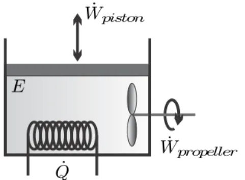
The transfer of energy by work and heat will be formulated in the first law of thermodynamics. For example, we may do work moving the propeller and agitate a fluid, which increases the temperature of the fluid due to friction, but we will never observe a fluid at rest suddenly start moving a propeller and do work (e.g. lifting a weight), see fig.
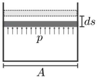
Mechanical State Properties
The pressure of the substance can be measured as the force required to hold a piston in place divided by the surface area of the piston. Usually we will only be interested in the absolute speed V, the SI unit is meters per second.
Extensive and Intensive Properties
A mass element's velocity vector is defined as its directed displacement per unit of time.
Specific Properties
Molar Properties
Inhomogeneous States
Processes and Equilibrium States
Quasi-static and Fast Processes
If the manipulation that causes a quasi-static process is stopped, the system is already in an equilibrium state and no further changes will be observed. If the manipulation that causes the non-equilibrium process is stopped, the system will undergo changes until it reaches its equilibrium state.
Reversible and Irreversible Processes
When the manipulation is rapid, so that the system does not have time to reach a new equilibrium state, it will be in a non-equilibrium state. The equilibrium process occurs while no manipulation takes place, i.e. the system is left to itself.
Temperature and the Zeroth Law
Thermometers and Temperature Scale
Gas Temperature Scale
The ideal gas temperature scale satisfies all requirements of the thermodynamic temperature scale that follows from the second law, and it coincides with the thermodynamic Kelvin scale. For convenience, temperatures are quite often given on the Celsius scale, but many thermodynamic equations require the thermodynamic temperature in Kelvin.
Thermal Equation of State
23.6, we will learn about the third law of thermodynamics, which, simply put, states that absolute zero≡0 K cannot be reached. Most often the same symbol, T, is used for temperatures on each scale, care must be taken not to get confused.
Ideal Gas Law
The number of moles of mass is related asn=m/M, so the ideal gas equation can also be written in another form, with the universal gas constant.
A Note on Problem Solving
Example: Air in a Room
Example: Air in a Refrigerator
More on Pressure
When the fastener is removed from the piston, the piston moves up, and the spring is compressed. The mass of the balloon, basket included, but without the gas filling, is mB = 500 kg.
Conservation of Energy
This equation states that the change of energy of the system over time (dE/dt) is equal to the energy transferred by heat and work per unit time (˙Q−W˙. All contributions to the first law (3.1) , i.e. energy , work and heat, are discussed in detail in the following paragraphs.
Total Energy
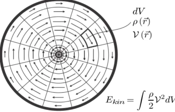
Kinetic Energy
Potential Energy
Internal Energy and the Caloric Equation of State
Work and Power
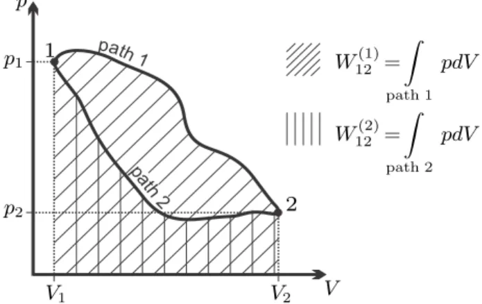
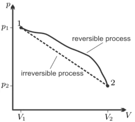
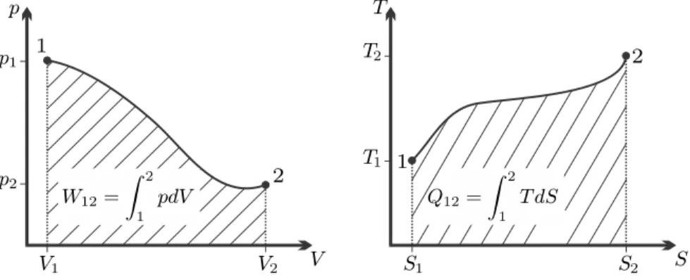
In quasi-static (or reversible) processes, the system goes through a series of equilibrium states that can be represented in suitable diagrams. In general, there can be several work interactions ˙Wj of the system, then the total work for the system is the sum of all contributions; for example for power.
Exact and Inexact Differentials
Heat Transfer
By convention, heat transferred to the system is positive, heat transferred from the system is negative. In general, there can be several heat interactions ˙Qkof the system, then the total heat for the system is the sum of all contributions; eg. for the heating rate.
The First Law for Reversible Processes
The Specific Heat at Constant Volume
For incompressible liquids and solids, the specific volume is constant, v = const, and the specific heat is a function of temperature alone. Interestingly, even for ideal gases, the specific heat appears to be a function of temperature alone, both experimentally and from theoretical considerations.
Enthalpy
While its internal energy depends only on temperature, the enthalpy of an incompressible substance (constant specific volumev) depends on temperature and pressure. With h0 as the enthalpy at the reference point (T0, p0), it becomes the enthalpy for an incompressible solid or liquid with constant specific heat. 3.25) Note that no substance is truly incompressible, usually the specific volume changes at least a little.
Example: Equilibration of Temperature
For solids and incompressible liquids (v = const.), the specific heats at constant pressure and constant volume agree, since. However, our experience, defined in the zeroth law, tells us that the final temperatures agree: TA=TB=T.
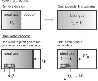
Example: Uncontrolled Expansion of a Gas
Example: Friction Loss
Example: Heating Problems .1 Heating of Water
Heating of Water with Heat Loss
Our sense of cold or hot is not a sense of temperature, but rather a sense of heat transfer. When we touch an object with a large heat transfer coefficient, a large amount of heat is exchanged between our hand.
Isochoric Heating of an Ideal Gas
A greater amount of heat can be transferred to our hand from an object with a large thermal massmc.
Isobaric Heating of an Ideal Gas
It is observed that after 10 minutes the temperature of the ice cream has dropped from T1=−2◦C to T2=−18◦C. Temperature at the end of expansion and heat exchange with the environment.
The Second Law
Entropy and the Trend to Equilibrium
The process from the initial equilibrium state to the final equilibrium state takes some time. Since entropy increases only before the equilibrium state is reached, the latter is the maximum entropy.
Entropy Flux
Entropy in Equilibrium
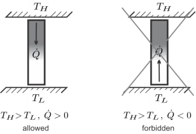
So far, entropy and the coefficients β and γ in the entropy flux have not been determined. In particular, it will be seen that the entropy flux term βQ˙ = ˙Q/T is related to limiting the direction of heat transfer: heat flows from hot to cold, not the other way around.
Entropy as Property: The Gibbs Equation
T-S-Diagram
The entropy s(T, v) follows from this either by replacing the pressure with the ideal gas equation (p=RT /v) or by integration (4.12) as (for constant specific heat).
The Entropy Balance
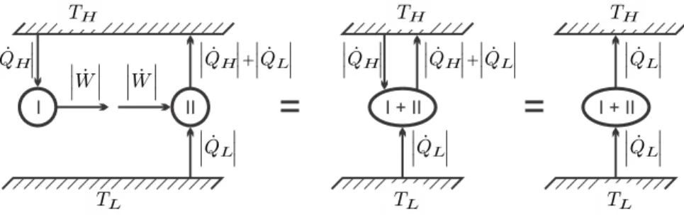
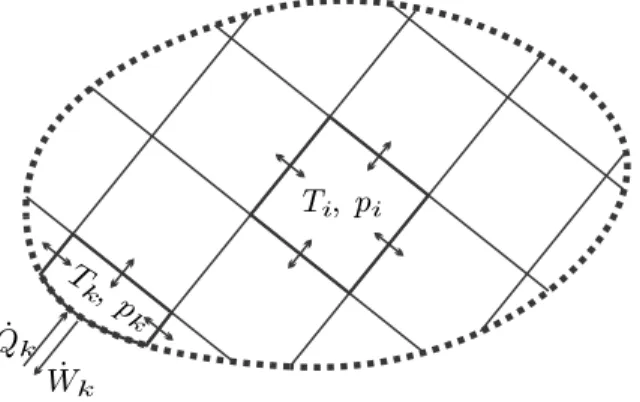
In the above, ˙Qk is the heat transferred across a system boundary with temperature Tk. Since energy is conserved, the internal exchange of heat and work between subsystems cancels out in the law of conservation of energy (4.23).
The Direction of Heat Transfer
Extending the argument shows that the internal exchange of heat and work between subsystems sums up to zero, so that only exchange with the surroundings, denoted by subscriptk, appears in (4.23). Clausius' original derivation of the second law is based on the statement that heat will go from hot to cold by itself, but not vice versa.
Internal Friction
Furthermore, the gearbox is in thermal contact with the environment from which it receives the heat ˙Q. The statement of the first law can be read directly from the figure: Energy flow in (arrows pointing towards the gearbox) must equal energy flow out (arrows out of the gearbox).
Newton’s Law of Cooling
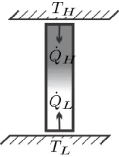
Only when the temperature difference is infinitely small, i.e. TH =TL+dT, the generation of entropy can be ignored and heat transfer can be considered as a reversible process. This can be seen as follows: For infinitesimal dT, the entropy generation rate becomes ˙Sgen = αA.
Zeroth Law and Second Law
Heat transfer was introduced as energy transfer due to temperature change with heat passing from hot to cold, Newton's laws of cooling state that as a result of temperature change you will observe a response, namely heat flow. With Newton's law of cooling it is easy to see that heat transfer over finite temperature changes is an irreversible process. 4.36).
Example: Equilibration of Temperature
Example: Uncontrolled Expansion of a Gas
The total entropy change follows from the ideal gas entropy (with constant specific heat), Eq. Since in this process the temperature of the ideal gas remains unchanged, the increase in entropy is attributed only to the increase in volume: by filling a larger volume V2, the gas assumes a state of higher entropy.
What Is Entropy?
It is instructive to compare the number of realizations for the two cases for which we find. In addition, inhomogeneous distributions are quite unlikely, since the number of homogeneous distributions is much greater than the number of highly inhomogeneous distributions.
Entropy and Disorder
In Statistical Thermodynamics it is found that in equilibrium states the distribution of microscopic energies between particles is exponential, Aexp. You could say that the exponential function itself is an ordered function, so the equilibrium states are less disordered than non-equilibrium states.
Entropy and Life
The factor A must be chosen so that the sum of all particles gives the internal energy U. Moreover, at lower temperatures the exponent is narrower, the energies of microscopic particles are limited to lower values, and one could say that the equilibrium states at low temperatures are more ordered than at high temperatures balance.
The Entropy Flux Revisited
The other half of the container is emptied and the container is well insulated. From the first and second laws, determine the final temperature T2, the volume of the larger container and the resulting entropy.
Energy Conversion
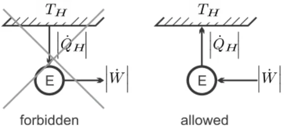
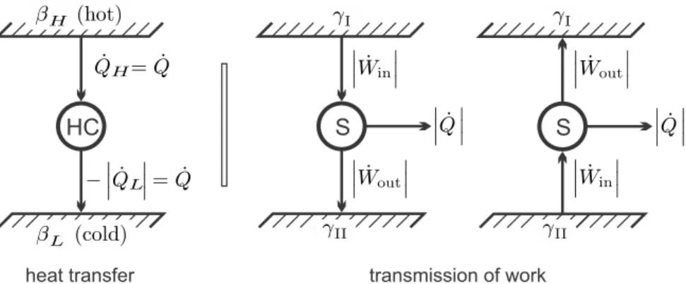
However, for the overall current evaluation, they are not of concern, and therefore the resulting setup is as simple as shown in Fig. However, in the following figures, we will use the absolute values of heat and work, and the direction of the flows will be indicated by the directions of the arrows.
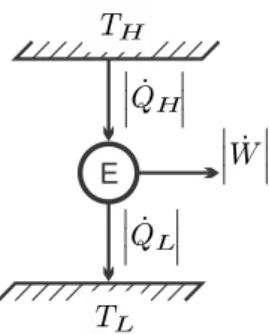
Heat Engines
Instead, the engineering task is to minimize the entropy build-up in the system in order to achieve the best possible engine performance. The above is summarized in two statements: a) The thermal efficiency of a fully reversible engine operating between two reservoirs is independent of the engine design; it is given by the Carnot efficiency ηC.
The Kelvin-Planck Statement
Since it is calculated from general considerations, its value is completely independent of the details of the engine, that is, it does not depend on the working fluid used, nor on the realization of the engine. The Carnot efficiency is a universal limit to the thermal efficiency of any engine operating between two reservoirs at TH, TL.
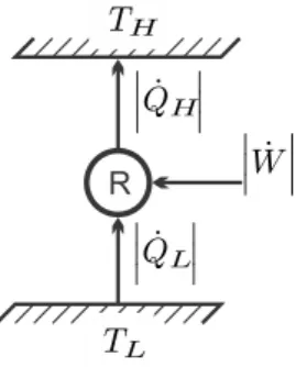
Refrigerators and Heat Pumps
For heat pump systems, one is interested in the work required regarding the heat supply ˙QH to the warmer reservoir. 5.10) Since TS˙gen ≥0, each generation of entropy within a refrigeration or heat pump system increases labor demand. and therefore operating costs. The theoretical limit for the work of the cooling and heat pump systems is obtained for fully reversible motors, for which ˙Sgen = 0.
Kelvin-Planck and Clausius Statements
Thermodynamic Temperature
The Kelvin scale assigns the value eTT r = 273.16 K to this unique point, which can be easily reproduced in laboratories. 8.2, when we explicitly calculate the thermal efficiency of a Carnot cycle operating with an ideal gas.
Perpetual Motion Engines
Reversible and Irreversible Processes
Since the heat added to the environment, Q21, cannot be completely converted into the work needed to push, W21, the changes remain in the environment. Thus, process 2-1 withdraws work W21 from the surroundings and transfers heat Q21 to the surroundings.
Internally and Externally Reversible Processes
Irreversibility and Work Loss
5.17) This equation generalizes the findings of the previous sections to arbitrary processes in closed systems: The generation of entropy in irreversible processes reduces the work output of work-producing devices (where ˙W > 0, e.g. heat engines) and increases the work requirement of work-consuming appliances (where ˙W < 0, e.g. heat pumps and refrigerators). It is an important engineering task to identify and quantify the irreversible work losses, and to reduce them by redesigning the system, or using alternative processes.
Examples
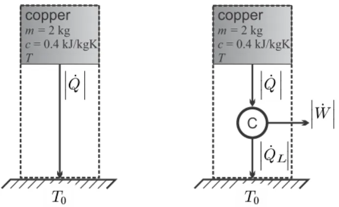
- Entropy Generation in Cooling
- Work Generation in Cooling
- Perpetual Motion Engines
- A Heat Engine
- Refrigerator
- Heat Pump with Internal and External Irreversibilities
8 kW the first law is not fulfilled—. the device is a perpetual motion machine of the first kind. Calculate the heat rejected, the thermal efficiency, the entropy generation rate, and the work loss for irreversibilities.
State Properties and Their Relations
Inversion of the caloric equation of state u(T, v) for temperature yields temperature as a function of energy and volume,T(u, v). Taking the latter into account in the entropy expression s(T, v) yields entropy as a function of energy and volume, s(u, v).
Phases
The thermal and caloric equations of state, p(T, v) and u(T, v), must be determined in careful measurements, the measurement of the latter being based on the first law. Entropy must be determined from the thermal and caloric equations of state through integration of the Gibbs equation, which gives a differential relation between properties and holds for all simple substances of the form.
Phase Changes
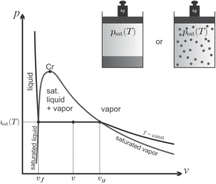
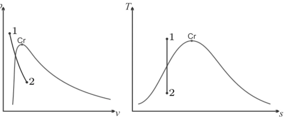
At the critical point, all properties between vapor and liquid match, and above the critical point only one phase exists, one speaks of supercritical fluid. Away from the saturation lines, the substance will only be in one of the phases as shown in the figure.
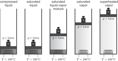
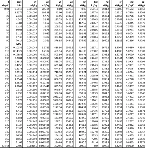
Saturated Liquid-Vapor Mixtures
Other extensive amounts, e.g. internal energy U, enthalpyH or entropy S, is calculated from the specific properties of the saturated liquid and vapor states, just like the volume. The specific energy, enthalpy, entropy of the saturated liquid is denoted asuf(T),hf(T),sf(T), and the saturated vapor asug(T),hg(T),sg(T).
Identifying States
A state of given pressure, for which another property (v oruor hor s) is known, liquid is compressed to.
Example: Condensation of Saturated Steam
6.12, the isochoric process at the lowest temperature is a vertical line down from the saturated vapor curve, and final state 2 lies in the two-phase region between the saturation lines. Final state 2 is in the two-phase region (mixture of saturated liquid and saturated vapor).
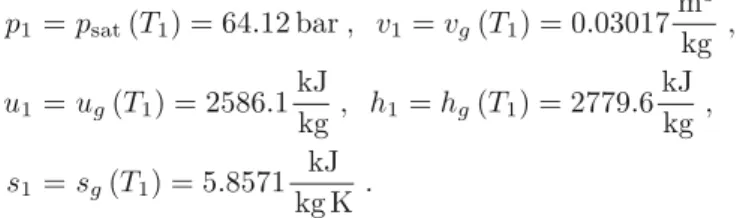
Superheated Vapor
The required value for entropy cannot be found in the table, but lies between the given values. The closest values above and below the required value of 2= 7.3549kg KkJ in the table are.
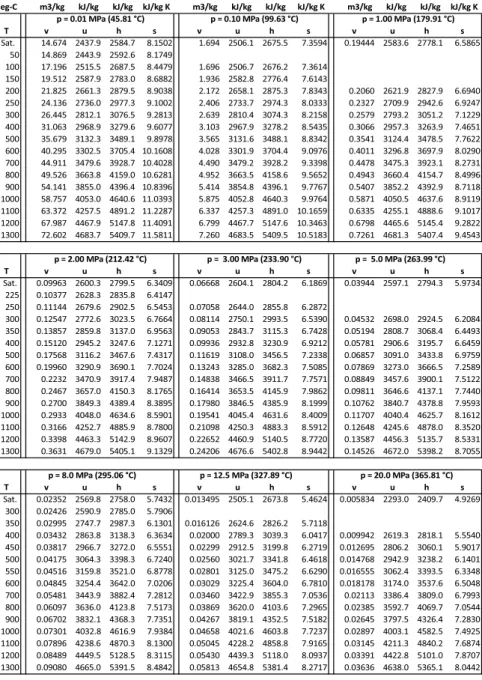
Compressed Liquid
Combining both by eliminating uf(T), we find the approximation for the enthalpy of compressed fluid as. With this approximation, isobaric lines for the compressed fluid in the T-s diagram lie on the saturated fluid line.
The Ideal Gas
The value of the reference entropy (T0, p0) can be obtained from the third law, which will be discussed later (Sec. 23.6). When one is not interested in entropy as a function of T and p, but as a function of T and v, the ideal gas law can be used to eliminate pressure.
Monatomic Gases (Noble Gases)
Specific Heats and Cold Gas Approximation
Real Gases
For large values of the specific volumev the equation reduces to the ideal gas law. 16.8, where it will be seen that the equation gives a good qualitative description of real gas effects and liquid-vapor phase change.
Fully Incompressible Solids and Liquids
The volume of the container is then fixed and the steam is cooled further until the temperature is 20◦C (position 3). Then the volume of the container is fixed and the heating continues until all the liquid has just evaporated (position 3).
Standard Processes
Basic Equations
We calculate the process curve of an isochoric process on the T-s diagram for an ideal gas with constant specific heat. Thus, for an ideal gas, the isochoric process in the T-s diagram follows an exponential, as shown in the T-s diagram.
Isobaric Process: p = const., dp = 0
From the Gibbs equation and the caloric equation of state we find for the isochoric process. 7.11).
At constant specific heat, the entropy is given by (6.27), which for an isentropic process gives
Isothermal Process: T = const, dT = 0
Polytropic Process (Ideal Gas): pv n = const
Summary
Examples
- Isochoric Process for Ideal Gas
- Isochoric Heating of Water
- Isobaric Heating of Ideal Gas
- Isobaric Cooling of R134a
- Isentropic Compression of Ideal Gas
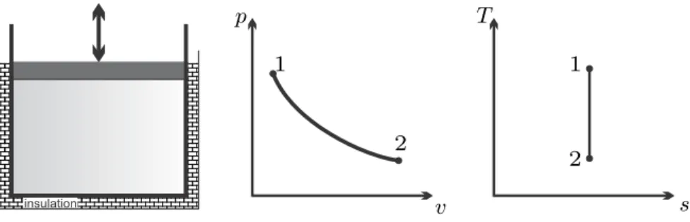
- Reversible and Irreversible Adiabatic Expansion
- Isentropic Expansion of Compressed Water
- Isothermal Expansion of Steam
- Polytropic Process
We calculate the final state, the heat supplied and the work done by the gas. Calculate the work and heat transfer per kg of air when the compression process is (a) isothermal, (b) isentropic, (c) isentropic with constant specific heat (approximation of cold air), (d) polytropic.
Thermodynamic Cycles
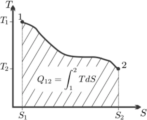
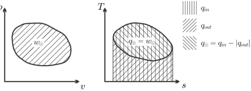
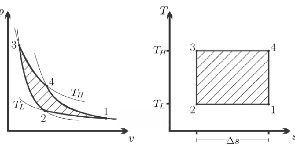
In the p-v diagram, the net work is just the area enclosed by the process curve as shown in the figure. Similarly, the net heat exchanged for a reversible cycle is the area enclosed by the cycle in the T-s diagram.
Carnot Cycle
Of course, due to irreversibilities, the actual engine will have an efficiency below the Carnot efficiency. In fact, one does not try to build engines that follow the Carnot cycle for practical applications.
Carnot Refrigeration Cycle
In principle, you could try to design an engine that would follow the Carnot cycle. Of course, these have efficiencies below the Carnot efficiency due to unavoidable internal and external irreversibilities.
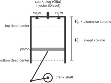
Internal Combustion Engines
The hot combustion gas expands in the third stroke, as the piston returns to bottom dead center. During strokes I and IV, the valves are open, and the mass in the cylinder changes.
Otto Cycle
The simplified analysis shows that the compression ratio r is the most important parameter for the evaluation of the Otto cycle. Under the cold air assumption, the thermal efficiency depends only on the compression ratio and increases as the compression ratio increases.
Example: Otto Cycle
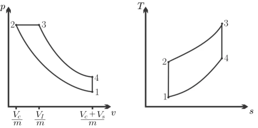
Diesel Cycle
However, the diesel cycle allows significantly higher compression ratios than the Otto cycle, which is why it has a greater efficiency. From the p-v diagram we can see that in a Diesel cycle the maximum pressure is maintained for a longer period, unlike the Otto engine where.
Example: Diesel Cycle
Because of this, diesel engines have to be built more strongly, which is the main reason why they are more expensive. This is somewhat lower than the efficiency under the cold air approximation, which is η = 1−rk−11.
Dual Cycle
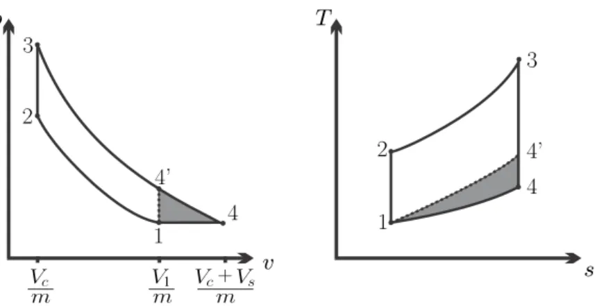
Atkinson Cycle
Based on the data obtained, discuss the feasibility of the process (except that it would be impossible to build a fully reversible engine). Determine the mass of air in the cylinders and net power output of the engine when running at 4500 rpm.
Flows in Open Systems
In an open system, non-equilibrium is maintained by the exchange of mass, heat and work with the surroundings.
Conservation of Mass
The macroscopic mass flow through the finite section A results from the integration of all surface elements. At the final cross-section, we would expect spatial variations of the density ρ and the velocity V⊥ across the cross-section, which should be taken into account in the integral.
Flow Work and Energy Transfer
W˙ flow , (9.7), where the sum must be taken over all flows that cross the system boundary. 9.8) Enthalpyh=u+pρ arises through the combination of convective transport of internal energy and flow work. Explicitly accounting for mass flows leaving and entering the system becomes the 1st law - the energy balance - of the general open system.
Entropy Transfer
Open Systems in Steady State Processes
One Inlet, One Exit Systems
In the p-v-diagram, wrev12 is the area to the left of the process curve, see figure. Correspondingly, the specific reversible heat, i.e. heat per unit mass flowing through the device.
Entropy Generation in Mass Transfer
In a T-s diagram, q12rev is the area under the process curve, just as in a closed system. Then A is the cross section of the porous medium considered, and β is a coefficient of permeability.
Adiabatic Compressors, Turbines and Pumps
The system includes the heat transfer to a reservoirR, the system boundary is shifted. thin lines 1-2s), while in irreversible adiabatic compressors and turbines the entropy has to grow (dotted lines 1-2s), as illustrated in the figure.
Heating and Cooling of a Pipe Flow
Applying the second law to the reservoir-boundary system, where the temperature is TR, gives the yield. Heat exchange between flows in closed and open heat exchangers will be discussed in Sects.
Throttling Devices
Adiabatic Nozzles and Diffusers