TOWARDS A ROBOT ASSISTED BREAST BIOPSY SYSTEM By
Vishnu Mallapragada Dissertation
Submitted to the Faculty of the Graduate School of Vanderbilt University
in partial fulfillment of the requirements for the degree of
DOCTOR OF PHILOSOPHY in
Mechanical Engineering December, 2008 Nashville, Tennessee
Approved:
Professor Nilanjan Sarkar Professor Eric Barth Professor George E. Cook Professor Michael Goldfarb
Professor Tarun K. Podder
ACKNOWLEDGEMENTS
I would like to thank my advisor, Professor Nilanjan Sarkar, for his guidance. He gave me the freedom to pursue my ideas while providing clear direction when I encountered road blocks. His insight and discussions helped me greatly during my doctoral work.
The members of my dissertation committee, Professors Michael Goldfarb, Tarun Podder, Eric Barth and George Cook have generously given their time and expertise to better my work. I thank them for their contribution.
This work would not have been possible without the help of Professor David Pickens. I would like to thank him for giving me access to the ultrasound equipment in the Radiology Imaging Research Laboratory.
I would like to express my gratitude to Professor Michael Goldfarb for letting me fabricate device components on the rapid prototyping machine.
It has been a pleasure working with my labmates in the Robotics and Autonomous Systems Laboratory. I’m forever grateful to my parents for their love, encouragement and support. I have shared the best and worst moments of this journey with my wife. Her love, sacrifice, patience and good humor helped me persevere through many sleepless nights.
TABLE OF CONTENTS
Page
ACKNOWLEDGEMENTS ... ii
LIST OF TABLES ...v
LIST OF FIGURES ... vi
LIST OF ABBREVIATIONS ... ix
Chapter I. INTRODUCTION ...1
II. MANIPULATION OF DEFORMABLE OBJECTS ...6
Techniques for Deformable Object Manipulation ...7
Geometric Arrangement of Robotic Fingers ...8
Target Position Control ...11
Passivity Based Control ...17
Target Position Error...17
Passivity Observer ...19
Passivity Controller ...21
Passivity Proof ...22
Servo Loop Controller ...23
Choice of E0 ...24
III. ROBOTIC IMAGE GUIDED BREAST BIOPSY SYSTEM ...27
Review of Interventional Robotic Systems...30
Techniques to Compensate for Needle – Target Misalignment ...30
Robotic Systems for US Image Acquisition ...31
Design of Robotic Image-Guided Breast Biopsy System ...34
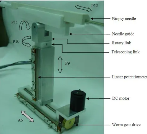
Design of Robotic Manipulation Mechanism ...35
Design of Autonomous Image Acquisition System ...40
Design of Needle Guidance System ...43
Integrated System...44
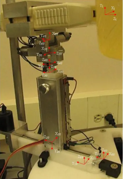
Forward Kinematics of RIBBS ...48
Forward Kinematics of US Imaging System ...49
Forward Kinematics of Needle Guidance System ...51
Global Reference Frame for RIBBS ...53
RIBBS Control Architecture ...54
Controller for US Image Acquisition System ...54
Hybrid Supervisory Controller ...56
Planner ...63
Safety ...66
IV. EXPERIMENTAL RESULTS...67
Phantom Properties ...67
Deformable Object Manipulation ...71
Experimental Setup for Planar Target Manipulation ...72
Regulation ...73
Tracking ...86
Error Analysis of Target Positioning During Planar Manipulation ...89
Needle – Target Alignment During Breast CNB ...90
Needle Orientation in Global Reference Frame ...90
Experimental Setup for Needle Insertion ...93
Target Manipulation During Needle Insertion ...96
Targeting Accuracy During Breast CNB ...109
V. CONCLUSION ...111
Appendix A. PHANTOM SPECIFICATIONS ...114
REFERENCES ...117
LIST OF TABLES
Table Page
3.3.1.1 D-H parameters for US device ...50
3.3.2.1. D-H parameters for needle guidance device ...52
3.4.2.1. Events for high level controller...60
3.4.2.2. Supervisory control strategy ...62
3.4.2.3. Preferred clinician action based on system state ...63
4.1.1. Phantom specifications ...69
4.1.2. Actuator motion characteristics for phantom compression trials ...69
4.1.3. Young’s modulii of phantoms ...70
4.1.4. Young’s modulus of breast tissue ...71
4.2.4.1. Error in target positioning using PBC ...89
4.3.1.1. Relative measurement error of needle tip ...93
4.3.4.1. Targeting accuracy during needle insertion ...110
A.1. Specifications for phantoms used in experiments ...116
LIST OF FIGURES
Figure Page
1.1. Needle insertion schematic for breast CNB ...4
2.2.1. Robotic fingers in contact with a deformable object ...9
2.3.1. Manipulation for target position control using robotic fingers ...11
2.3.2. Control Structure for manipulating deformable objects ...12
2.3.3. M-port network ...13
2.3.4. Network representation of deformable object manipulation ...14
2.4.1. Network representation of deformable object manipulation with PBC ...20
3.1. Finite element modeling of needle insertion in elastic tissue ...28
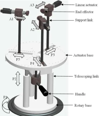
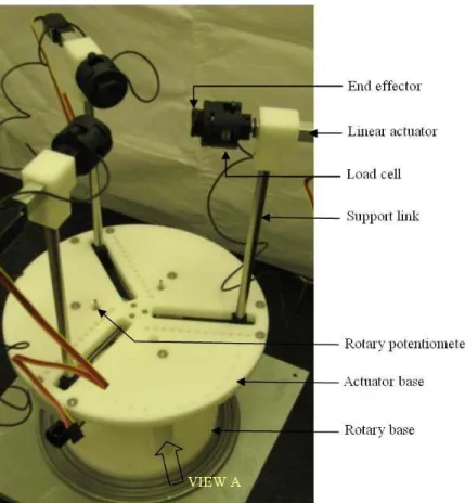
3.2.1.1. Design of manipulation mechanism...37
3.2.1.2. Perspective view of manipulation mechanism ...38
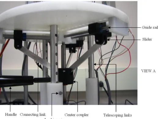
3.2.1.3. (View A) Mechanism for coupled radial motion of robotic fingers ...38
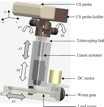
3.2.2.1. Design of image acquisition system ...42
3.2.2.2. Image acquisition system ...42
3.2.3.1. Needle guidance device ...43
3.2.4.1. Integrated design of RIBBS ...46
3.2.4.2. RIBBS testbed with breast phantom ...46
3.2.4.3. RIBBS architecture ...47
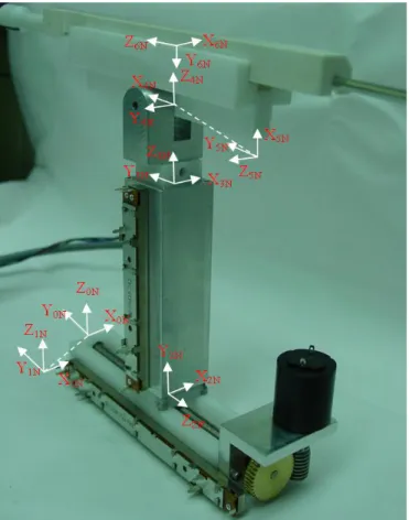
3.3.1.1. Coordinate frame assignment for US device ...49
3.3.2.1. Coordinate frame assignment for needle guidance device ...52
3.3.3.1. Coordinate frame assignment for RIBBS ...53
3.4.2.1. Hybrid control architecture ...57
3.4.2.2. Supervisory controller ...61
3.5.1. Control structure for minimizing needle - target misalignment ...64
3.5.2. Needle - target alignment during breast CNB ...64
4.1.1. Phantom stress-strain curves for Trial 1. ...70
4.2.1.1. Experimental setup for planar manipulation of phantoms ...72
4.2.2.1. Target position response for different gains (a) X displacement (b) Y displacement ...75
4.2.2.2. Target position response for different phantoms (a) X displacement (b) Y displacement ...77
4.2.2.3. Target position response with step disturbance (a) X displacement (b) Y displacement ...79
4.2.2.4. Desired and actual velocities of robotic fingers without PO/PC (a) Desired and actual velocities (b) Actual velocities ...82
4.2.2.5. Net energy output of outer loop controllers without PO/PC. Inset shows a close up view of the energy plot from 0 - 4 seconds ...83
4.2.2.6. Net energy output of outer loop controllers with PO/PC. Inset shows a close up view of the energy plot from 0 - 4 seconds ...85
4.2.2.7. Desired and actual velocities of three robotic fingers with PO/PC ...86
4.2.3.1. Trajectory tracking with passivity based controller (a) X displacement (b) Y displacement ...89
4.3.1.1. Experimental setup for determining measurement error ...91
4.3.2.1 Experimental setup for target manipulation during needle insertion ...95
4.3.3.1 Target and nominal needle paths during needle insertion (a) 3D (b) projection onto the XY (horizontal) plane ...98
4.3.3.2. Target position response during needle insertion (a) X displacement (b) Y displacement ...99
4.3.3.3. Target and nominal needle paths during 3D needle insertion...101
4.3.3.4. Signals for enabling/disabling supervisory controller states ...102
4.3.3.5. Target position response during needle insertion (a) X displacement (b) Y displacement ...103
4.3.3.6. Joint coordinates of US image acquisition device ...104
4.3.3.7. Target and nominal needle paths during 3D needle insertion...106
4.3.3.8. Signals for enabling/disabling supervisory controller states ...107
4.3.3.9. Target position response during needle insertion (a) X displacement (b) Y displacement ...108
4.3.3.10. Joint coordinate of US image acquisition device ...108
A.1. Schematic of material distribution in inhomogeneous phantoms ...114
A.2. Central and peripheral regions in phantoms ...115
LIST OF ABBREVIATIONS
3D Three Dimensional
US Ultrasound
FNAB Fine Needle Aspiration Biopsy
CNB Core Needle Biopsy
PBC Passivity Based Control
2D Two Dimensional
P Proportional
PI Proportional-Integral
PID Proportional-Integral-Derivative
PO Passivity Observer
PC Passivity Controller
PBC Passivity Based Control
RIBBS Robotic Image-guided Breast Biopsy System
DOF Degrees Of Freedom
DOA Degrees Of Actuation
PPM Pulse Position Modulation
D-H Denavit-Hartenberg
SC Supervisory Controller
DES Discrete Event System
LED Light Emitting Diode
WRLS Weighted Recursive Least Squares
EM ElectroMagnetic
CHAPTER I
INTRODUCTION
Subcutaneous insertion of a surgical device is common in clinical practice. In minimally invasive procedures such as hollow core needle biopsy, percutaneous tumor ablation etc., a surgical instrument is inserted into soft, inhomogeneous tissue in order to sample or remove a target (in this work the word target is used to refer to a tumor, a lesion or just a suspected region of tissue). In such procedures it is critical to position the instrument tip precisely at the target. Accurate needle placement at the target location is essential to reduce false negative results during biopsies. “While many factors are important to achieve local tumor control of a targeted lesion when using percutaneous image-guided ablation devices, the most important one is accurate placement of the device in the center of the targeted tumor.” [1]
Minimally invasive procedures have numerous benefits such as low cost, short operating time, quick recovery of patient etc. Despite these advantages, precise placement of a surgical needle at the target is challenging because of several reasons such as tissue heterogeneity and elastic stiffness, tissue deformation and movement, and poor maneuverability of the needle.
For procedures involving small diameter needles (such as the 18 – 25 gauge needles used for FNAB), heterogeneous nature of the tissue causes needle bending during insertion. For procedures involving large diameter needles (such as 10 – 14 gauge needles used for CNB) if the tip of the needle reaches interface between two different types of tissue, its further insertion will push the tissue, instead of piercing it, causing unwanted deformations. Tissue deformation causes the target to move away from the line of insertion of the needle
especially for deep seated targets. [2] describes a 3D finite element model of needle insertion in soft tissue. Results presented in [2] show that as the needle is inserted, large tissue deformation causes the target to move away from the path of the needle. Target motion can also be caused due to breathing or other involuntary movement of the patient. Since needle insertion point and needle orientation (in this work, the word orientation is used to refer to the six degrees of freedom of the needle) are chosen by assuming a straight line path to the target, needle bending or target motion causes error in placing the needle tip at the target location. In spite of the considerable skill of a clinician, it is difficult to achieve accurate and consistent results through manual compensation of needle - target misalignment.
Manually performed US guided needle breast biopsy and stereotactic breast biopsy have false negative rates of 1.7% and 8.9% respectively [3]. US guided procedures have lower false negative rates due to availability of real time image guidance. One of the main causes of false negative results is suboptimal sampling [4]. Suboptimal sampling is a direct consequence of target motion due to patient movement and tissue deformation. False negative rate for breast biopsy is fairly low, since, in clinical practice several insertions are performed to achieve good needle – target alignment. It has been noted that approximately five insertions are required to align a 3 mm target with manual needle insertion [5].
Retargeting (retraction of the needle and reinsertion due to needle – target misalignment) is also common for stereotactic breast biopsies. Retargeting and multiple insertions cause excessive bleeding which obscures the guiding images and causes significant discomfort to the patient. Retargeting is also fatiguing for the clinician and increases procedural time which is directly related to cost of the procedure.
In order to overcome the above limitations, significant research effort is being made to
investigate techniques that can address the problem of needle - target misalignment during needle insertion. In [6]-[8], steerable devices are presented that allow the clinician to steer the tip of the needle towards the target during insertion. A visually controlled needle-guiding system is developed in [9] for automatic or remote controlled percutaneous interventions. In the automated mode, the needle insertion path is updated based on image feedback to the needle-guiding system. Though these systems potentially reduce the number of insertions required to sample the target, maneuvering a needle inside the body causes tissue damage. In [10][11], a finite element model is used to predict movement of the target. Needle path is planned based on this prediction to accurately sample the target. To get an accurate prediction of the movement of the target, finite element analysis requires the geometric model and mechanical properties of the anatomical structures. In addition, finite element computation is not real-time. For example, in [10], the average time for computation is 29 minutes.
In this work, a new paradigm for image guided minimally invasive procedures is presented. In this approach a robotic system will be able to position a target inline with a surgical device during insertion in a safe and accurate manner. The system developed is for automating US guided breast CNB although much of the system development could be adapted to other real time imaging modalities and for performing FNAB, ablation etc
During US guided breast CNB a clinician inserts a needle through an incision to remove a tissue sample. A schematic of needle insertion in a breast is shown in Fig. 1.1. The two dimensional plane of the figure represents a horizontal plane passing through the target (the target mass in Fig. 1.1). In the figure, a simplified anatomy for the breast is shown. In reality, breast tissue is inhomogeneous and its biomechanical properties are nonlinear. Hence, if the
tip of the needle reaches the interface between two different types of tissue, its further insertion will push the tissue, instead of piercing it, causing unwanted deformations. These deformations move the target away from its original location, as shown in Fig. 1.1.b. The robotic system which consists of a set of actuators positioned around the breast applies force on the surface of the breast based on the image of the target to guide the target towards the line of insertion of the needle (Fig 1.1.c). This approach is independent of the specific surgical device used for performing the procedure. The accuracy of this system is demonstrated with a vacuum assisted biopsy needle. The system can autonomously position a target at a desired location (typically in the path of the needle) with a high degree of accuracy.
Fig. 1.1. Needle insertion schematic for breast CNB.
This robotic device has the following potential advantages: (a) Success rate (defined by the number of insertions required at a particular biopsy site to successfully sample the target tissue) of the procedure will be increased since the target is accurately positioned inline with the needle. (b) Since the number of insertions required is expected to be less, it will reduce fatigue of the clinician and patient discomfort. (c) The entire procedure is predicted to be
fast, making it clinically viable. (d) Since the needle is not steered inside the breast, and the number of insertions reduced, tissue damage is also potentially minimized and the structural integrity of the tissue specimen is preserved. (e) Geometric and mechanical properties of the breast are not required for precise positioning of the target. (f) By improving accuracy of biopsy, it will potentially enhance the diagnostic outcome by reducing the false negative rate.
This dissertation is organized as follows: Chapter II casts the needle – target alignment problem in a control framework and develops a PBC approach for manipulation of deformable objects (soft tissue is a specific instance of a deformable object). Chapter III develops the design of a integrated robotic system for automating US guided breast CNB.
This system automates and integrates needle – target alignment, image acquisition and processing, and US probe motion to provide comprehensive assistance for performing breast CNB. Chapter IV presents experimental results on phantoms with varying elastic properties to verify validity of the approach. This chapter also presents a discussion on the targeting accuracy of this technique. Chapter V describes the contributions of this work.
CHAPTER II
MANIPULATION OF DEFORMABLE OBJECTS
Precise position control of a target embedded in soft tissue requires the ability to manipulate the soft tissue surrounding the target. The breast is a many layered organ consisting of various structures such as lobules, Cooper’s ligaments and connective tissue.
Biomechanical models of breast predominantly consist of two different types of tissue: fatty and glandular [12][10]. These tissues display viscoelastic response and in order to develop tractable mathematical models, researchers have assumed these tissues to be isotropic [14].
There is a lot of research in robotic grasping and manipulation of deformable objects with a wide range of applications [15][16]. In general, a deformable object is defined as an object whose degrees of freedom are characterized by viscoelastic interactions between the molecules. A deformable object changes its shape when an external force is applied [17].
Thus, breast tissue is a subset of a general class of inhomogeneous deformable objects and techniques used for robotic manipulation of deformable objects can be exploited for position control of a target embedded in soft tissue. Conversely, techniques developed for soft tissue manipulation can also be applied in other fields such as robotic assembly of flexible parts, fabric manipulation in textile manufacturing etc.
As will be discussed in Chapter III, ensuring needle – target alignment during breast CNB requires planar target position control. Hence, in this chapter, a technique for planar manipulation of deformable objects is developed.
Techniques for Deformable Object Manipulation
[19] presents an overview of research related to robotic grasping and manipulation of deformable objects with vision and tactile guidance. A general approach for position control of a nonlinear flexible structure is presented in [19]. The controller presented in [19]
guarantees global asymptotic stability of the closed loop. However, convergence of the output displacement (target point) to the desired position requires accurate knowledge of the stiffness of the system. A passivity based controller for flexible structures is presented in [20]. This controller uses nominal model information to construct an observer and maps the reconstructed state to an approximate passive output. The controllers developed in [19][20]
require information regarding the system model. In most cases, having a model of a nonlinear inhomogeneous deformable object is not feasible.
A simple PID controller is developed in [21] for manipulation and position control of deformable objects. Results presented in [21] show good convergence of the target points to the desired position but stability is not guaranteed due to noncollocation of the sensor and actuators. This controller is noncollocated since the desired configuration of the object is specified in terms of the states (target position) that are not directly actuated. PID controller design for a flexible link manipulator is developed in [22]. Due to distributed flexibility, a deformable object/manipulator is inherently an infinite dimensional system. But for control purposes, a finite dimensional model is obtained in [22] using system identification techniques. PID control gains are then chosen using H∞ control synthesis to guarantee robust performance.
An adaptive technique for control of a flexible structure with noncollocated sensors and actuators is presented in [23]. In [23], an adaptive PI controller with feedforward
augmentation is used to stabilize the system. Due to feedforward augmentation, only
boundedness of the tracking error is guaranteed. An impedance controller for a class of underactuated Euler-Lagrange systems based on energy shaping is presented in [24]. This approach is based on the fact that at equilibrium, there is an algebraic relationship (defined by a Jacobian) between the noncollocated and collocated variables. Design of a stabilizing controller is reduced to solving this algebraic equation for the noncollocated variable. [25]
presents a model independent passivity based approach to guarantee stability of a flexible manipulator with a noncollocated sensor-actuator pair. This technique uses an active damping element to dissipate energy when the system becomes active. A similar approach is developed in this chapter for manipulation of deformable objects with multiple robotic fingers.
Geometric Arrangement of Robotic Fingers
Before discussing the control system development, the goal is to determine the number of robotic fingers and their geometric arrangement necessary for planar position control of a target embedded inside the deformable object. Fig 2.2.1 shows the schematic of a robotic finger (a rigid link mechanism driven by a rotary or linear actuator) in contact with a deformable object. Without loss of generality, a circular deformable object is shown.
Fig. 2.2.1. Robotic fingers in contact with a deformable object.
In [21][26][27], the authors prove that one can control an internal point inside a deformable medium by applying force from the boundary. They further determine the number of robotic fingers required to position the target at an arbitrary location in the horizontal plane.
Result [27]: The number of manipulated (contact) points must be greater than or equal to that of the positioned (target) points in order to realize any arbitrary displacement.
In this case, the number of positioned points is one, since we are trying to control the position of just the target. Hence, ideally the number of manipulated points would also be one. But there are two practical constraints associated with this technique: (1) shear force on the surface should be minimized to avoid damage to the surface of the object; (2) the robotic finger is not rigidly attached to the surface, hence, only compressive forces directed into the object can be applied.
Thus this problem is more restrictive than [21][26][27] since the position of the target
needs to be controlled by applying only compressive force. However, there exists a general theorem in Mechanics [28] that determines the equivalent number of compressive forces that can replace one unconstrained force in a 2D plane.
Theorem [28]: A set of wrenches W can generate forces in any direction (in a plane) if and only if there exists a three-tuple of wrenches
{
w1,w2,w3}
whose respective force directions3 2 1,n ,n
n satisfy:
• Two of the three directions n1,n2,n3 are independent.
• A strictly positive combination of the three directions is zero, 0
, 0
3
1
>
∑
== i
i i
in α
α . (2.2.1)
The ramification of this theorem is that: (1) three robotic fingers are required; (2) the arrangement of the fingers should be such that the end points of their force direction vectors draw a non-zero triangle that includes their common origin point. With such an arrangement the target position can be controlled in a plane.
Target Position Control
Fig. 2.3.1. Manipulation for target position control using robotic fingers.
Fig. 2.3.1 shows a schematic of three robotic fingers in contact with a deformable object.
In this section, a control law for the robotic fingers is developed to guide a target from any point A to an arbitrary point B within the deformable object. At any given timestep, point A is the actual location of the target and point B is the desired location of the target. In Fig.
2.3.1, e (according to standard convention, letters in bold represent vectors) is the error vector pointing from A to B and indicates the error in target position. n1, n2 and n3 are unit vectors which determine the direction of force application of the robotic fingers with respect to the global reference frame G.
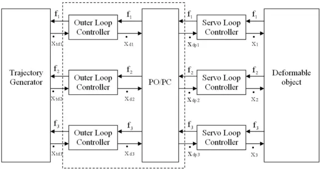
Fig. 2.3.2 is a schematic of the control structure for the entire system. In Fig. 2.3.2, Pd
is the position vector of point B and Pt is the position vector of point A. The position vector
Y
Ge
n 2
n3
n 1
Deformable Object
A B
X
GG
of point A is determined using image feedback. Error vector, e, is the difference between the desired and the actual target position. An outer loop controller (P control) determines the desired velocity for the actuators (which drive the robotic fingers), xd
•
, depending on the target position error. A servo loop controller (PI controller) acts on the error between the desired and actual actuator velocities,
•
x, to generate the actuator input, v. The desired control objective can be achieved with just the outer loop controller, the inner servo loop is used to add damping to the system [29]. The actuator velocities are determined using approximate differentiation of the position signals. The actuators drive the robotic fingers to apply a controlled external force, fc, on the surface of the object to guide the target towards the desired position. The control loop mitigates the effect of an external disturbance force, fn, on the target position.
Fig. 2.3.2. Control structure for manipulating deformable objects.
The stability of the above control system is analyzed using a passivity based approach.
First, the sign convention for all forces and velocities is defined such that their product is positive when power enters the system port. The following definition is used to analyze the passivity property of the system.
Definition [30]: The M-port network, NM(Fig. 2.3.3), with initial energy storage E(0) is passive if and only if,
[
( ) ( ) ( ) ( )]
(0) 0, 00
1
1 +⋅⋅⋅⋅⋅+ + ≥ ∀ ≥
∫
t f τ v τ fm τ vm τ dτ E t . (2.3.1)for all admissible forces
(
f1,⋅⋅⋅⋅⋅, fm)
and velocities(
v1,⋅⋅⋅⋅⋅,vm)
.Fig. 2.3.3. M-port network
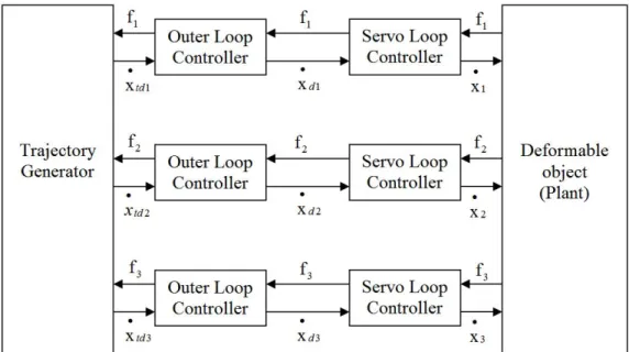
Similar to [31], energy is defined as the integral of the inner product between conjugate input and output, which may or may not correspond to physical energy. Equation (2.3.1) states that the energy applied to a passive network must be positive for all time. Fig. 2.3.4 shows a network representation of the energetic behavior of this control system. The block diagram in Fig. 2.3.3 is partitioned into four elements: the trajectory generator, outer loop controller, servo controller and plant. Each outer and servo loop controller pair corresponds to one actuator. Since three robotic fingers are used for planar manipulation, three controller pairs transfer energy to the plant.
Fig. 2.3.4. Network representation of deformable object manipulation.
The connection between servo loop controller and plant is a physical interface at which conjugate variables (fi, xi
•
; where fi is the force applied by actuator i and xi
•
is the velocity of actuator i) define physical energy flow between controller and plant. In this work, the subscript i refers to the ith finger. i takes values of 1, 2 and 3 representing the three fingers.
[
f1 f2 f3]
Tc=
f . (2.3.2)
⎥⎦ T
⎢⎣ ⎤
=⎡• • •
•
3 2
1 x x
x
x . (2.3.3)
The connections between trajectory generator and outer loop controller, and outer loop controller and servo loop controller, which traditionally consist of a one-way command information flow, are modified by the addition of a virtual feedback of the conjugate variable [31]. For the system shown in Fig. 2.3.4, output of the trajectory generator is the desired target velocity (xtdi
•
is the desired target velocity along direction of finger i) and output of
the outer loop controller is the desired actuator velocity (xdi
•
is the desired actuator velocity for actuator i).
⎥⎦ T
⎢⎣ ⎤
=⎡• • •
•
d3 d2
d1 x x
x
xd . (2.3.4)
For both connections, virtual feedback is the force applied by the robotic fingers. Integral of the inner product between trajectory generator output (xtdi
•
) and its conjugate variable (fi) defines “virtual input energy”. The virtual input energy is generated to give a command to the outer loop controller, which transmits the input energy to the plant through the servo loop controller in the form of “real output energy”. Real output energy is the physical energy that enters the plant (deformable object) at the point where the robotic finger is in contact with the object. Therefore the plant is a three-port system since three fingers manipulate the object.
The conjugate pair that represents the power flow is fi, xi
•
(force and velocity of finger i, respectively). The reason for defining virtual input energy is to transfer the source of energy from the controllers (outer and servo loop) to the trajectory generator. Thus the controllers can be represented as two-ports which characterize energy exchange between the trajectory generator and the plant. Note that the conjugate variables that define power flow are discrete time values and so the analysis is confined to systems having a sampling rate substantially faster than the system dynamics.
For regulating the target position during manipulation, x•tdi =0. Hence the trajectory generator is passive since it does not generate energy. However, for target tracking,
0 f and 0
x•tdi ≠ i ≠ . Therefore the trajectory generator is not passive because it has a velocity source as a power source. It is shown that even if the system has an active term, stability is
guaranteed as long as the active term is not dependent on the system states [32]. Therefore, passivity of the plant and controllers is sufficient to ensure system stability.
Elastic systems with collocated and compatible actuators and sensors are inherently passive [33]. Therefore, the plant is passive with respect to the pair fi and xi
•
, since this conjugate pair is collocated and compatible. It is known that a PI controller (servo loop controller) is output strictly passive with respect to the conjugate pair fi, -xi
•
[34]. However, the outer loop controller (P controller) may not be passive.
The virtual energy generated by the ith outer loop controller at the nth timestep, Ei(n), is given by
⎥⎥
⎦
⎤
⎢⎢
⎣
⎡
⎟⎟⎠
⎜⎜ ⎞
⎝
⎛ +
Δ +
=E (n-1) T f (n) Sat (x• (n)) Sat (x• (n)) n)
(
Ei i i 2 tdi 3 di . (2.3.5)
In the above equation, Ei(n-1) is the energy generated by the ith outer loop controller at the (n-1)th timestep; TΔ is the sampling time; fi(n) is the force applied by the ith finger at nth timestep, respectively; xtdi
•
(n) and xdi
•
(n) are the desired target and actuator velocities at nth timestep. The saturation functions, Sat2(q) and Sat3(q), are defined for any variable q, as follows:
⎩⎨
⎧
≤
= >
0 q 0
0 q if ) q
q (
Sat2 . (2.3.6)
⎩⎨
⎧
≥
= <
0 q 0
0 q if ) q
q (
Sat3 . (2.3.7)
Robotic fingers compress the tissue when the velocity of the finger is negative. Since the fingers transfer energy to the object only during compression, energy generated by the outer loop controller during compression is only considered for passivity analysis. The net energy
output of the ith outer loop controller at the nth timestep, Eneti(n), is given by
n)Eneti(n)=E0i +Ei( , (2.3.8)
where E0i is the initial stored energy of ith outer loop controller. The ith outer loop controller is not passive when Eneti(n) < 0. This can cause instability of the control system as shown in Fig. 2.3.2 and Fig. 2.3.4.
Passivity Based Control
A passivity control approach based on energy monitoring is developed for deformable object manipulation to guarantee passivity (and consequently stability) of the system. The basic idea is to use a passivity observer (PO) to monitor the energy generated by the outer loop controller (Fig. 2.3.4) and to dissipate excess energy using a passivity controller (PC) when the controller becomes active [31].
Target Position Error
Referring to Fig. 2.3.1, point A denotes the actual position of the target. The position vector of point A is given by
[
xt yt]
Tt =
P , (2.4.1)
where xt and yt are the position coordinates of point A in the global reference frame G. The desired target position is represented by point B whose position vector is given by
[
xtd ytd]
Td =
P . (2.4.2)
xtd and ytd are the desired target position coordinates. The desired target velocity is obtained by differentiating Eq. 2.4.2 with respect to time.
⎥⎦ T
⎢⎣ ⎤
=⎡• •
•
td ytd d x
p . (2.4.3)
xtd
•
and ytd
•
are the desired target velocities along XG and YG, respectively. The target position error, e, is
t
d P
P
e= − . (2.4.4)
Outer Loop Controller with Saturation Feedback Compensation The desired target velocity along the direction of actuation of the ith finger, xtdi
•
, is
i d n p ⋅
= •
•
xtdi , (2.4.5a)
where,
[
n1 n2 n3]
Ti =
n . (2.4.5b)
The error vector is resolved into components along the actuation directions as follows:
ni
e⋅
i =
e . (2.4.6)
A proportional – integral (PI) controller is used for the outer loop which generates the desired velocity for actuator i.
∫
∗• ∗
+
=K e K e dt
xdi pi i Ii i . (2.4.7)
Kpi is the proportional gain KIi is the integral gain for the ith outer loop controller. ei*
is the modified error with saturation feedback.
[
1 i i]
i i
i e e sgnSat (J ) J
e∗= + ⋅ − . (2.4.8)
Ji is the estimated target position
∫
•= x dt
Ji i . (2.4.9)
The saturation function, Sat1(q), is defined for any variable q, as
⎪⎩
⎪⎨
⎧
≥
≤
<
<
=
imax imax
imin imin
imax imin
1
l q if l
l q if l
l q l if q ) q (
Sat , (2.4.10)
where limin and limax represent the limits of motion of finger i. The result of using saturation feedback compensation (Eqs. 2.4.8 – 2.4.10) is that when finger i is within its limits of motion, xdi
•
is computed using Eq. 2.4.7. When finger i reaches its limit, x•di =0. There are several advantages in using such a scheme: (a) wear on the actuator is minimized; (b) wind up of the servo controller is eliminated, and (c) limits of finger motion can be chosen based on safety considerations, thereby reducing the risk of accidental damage to the object.
Passivity Observer
The passivity observer (PO) and passivity controller (PC) are implemented as shown in Fig. 2.4.1. The PO monitors the combined energy output of the three outer loop controllers.
When the energy becomes negative, PC dissipates energy from the controllers, based on the contribution of the individual controllers to the net energy output. Thus, passivity of the system (dotted box in Fig. 2.4.1) with three outer loop controllers and PO/PC is ensured.
Fig. 2.4.1. Network representation of deformable object manipulation with PBC.
Net energy output of an individual outer loop controller is given by
⎥⎥
⎦
⎤
⎢⎢
⎣
⎡
⎟⎟⎠
⎜⎜ ⎞
⎝
⎛ +
+ Δ
+
= f (n) Sat (x•∗ (n)) Sat (x• (n)) 1)
- n (
1) - n ( T f 1) - n ( E n) (
E i 2 tdi 3 di
i 2 i
i
i α , (2.4.11)
where, T
1) - n (
1) - n ( f
i 2
i Δ
α is the energy dissipated by the PC at the (n-1)th timestep.
1) - n (
1
αi is
the damping coefficient from Eq. 2.4.15. fi(n) Sat2(xtdi(n)) Sat3(xdi(n))⎟⎟ΔT
⎠
⎜⎜ ⎞
⎝
⎛ •∗ + • is the energy
generated at the nth timestep.
•∗
xtdi is the modified desired target velocity (along ni) with saturation feedback similar to Eq. 2.4.8.
[
1 i i]
tdi tdi
tdi x x sgnSat (J ) J
x•∗ = • + • ⋅ − . (2.4.12)
Saturation feedback is used for desired target velocity so that xtdi xtdi
∗ •
• = when robotic
finger is within limits and x•∗tdi =0 when the finger reaches the limit. When the finger reaches
its limit of motion, it does not follow the desired velocity command due to a mechanical stop.
In such a case, energy is not supplied to the plant. Saturation feedback mitigates the effect of the trajectory generator supplying energy to the controller when the finger manipulators do not transfer this energy to the plant.
The total energy output of the outer loop controllers is
∑
=+
= 3
1 i
i 0
obs(n) E E (n)
E , (2.4.13)
where, E0 is the combined initial energy of the controllers.
Passivity Controller
The passivity controller (PC) is a dissipative element that obeys the constitutive equation v
f =α [35], (2.4.14)
where f is force, v is velocity and α is the damping coefficient. The output of the outer loop controller is velocity and the input is force, which imposes admittance causality on the PC.
When the observed energy becomes negative, the damping coefficient is computed using the following relation (which obeys the constitutive Eq. 2.4.14):
⎪⎩
⎪⎨
⎧
≥
<
⋅ ⋅
− Δ
=
0 n) ( E if 0
0 n) ( E if n) ( n) r ( f T
n) ( E n)
( 1
obs obs 2 i
i obs
αi . (2.4.15)
In the above equation, ri is a weighting factor that determines the ratio of energy dissipation from each controller. ri is computed as follows:
[ ]
[ ]
∑
== 3
1 i
i 3
i 3 i
n) ( E Sat
n) ( E n) Sat
(
r . (2.4.16)
The computation for the weighting factor only considers active behavior of the (outer loop) controllers. When net output energy of a controller is positive, the corresponding term in Eq.
2.4.16 is zero. Therefore, PC dissipates energy only from the active controllers and the amount of energy dissipated at a port is directly proportional to the net output energy of the corresponding controller. Output of the PC is the desired velocity for ith finger, xdpi
•
, given by
n) (
n) ( x f
i di i
dpi = +α
•
•
x . (2.4.17)
When the ith (outer loop) controller is passive, xdpi di
•
• =x . When the ith controller is active
xdpi
•
is computed using Eq. 2.4.17.
Passivity Proof
The total energy of the system (dotted box in Fig. 2.4.1) with three outer loop controllers (at the nth timestep), E(n) is given by
∑ ∑
= =∗ •
•
⎥⎥
⎦
⎤
⎢⎢
⎣
⎡
⎟⎟⎠
⎜⎜ ⎞
⎝
⎛ +
⋅ Δ +
= 3
1 0
dpi 2 tdi
i
0 T f (k) Sat (x (k)) x (k)
E n) ( E
i n
k
. (2.4.18)
Substituting from Eq. 2.4.17,
∑ ∑
= =∗ •
•
⎥⎥
⎦
⎤
⎢⎢
⎣
⎡
⎟⎟⎠
⎜⎜ ⎞
⎝
⎛ + +
⋅ Δ +
= 3
1 0 i
di i 2 tdi
i
0 (k)
k) ( k) f ( x ) k) ( x ( Sat k) ( f T E
n) ( E
i n
k α . (2.4.19)
∑ ∑
= =∗ •
•
⎥⎥
⎦
⎤
⎢⎢
⎣
⎡
⎟⎟⎠
⎜⎜ ⎞
⎝
⎛ + +
⋅ Δ +
=
⇒ 3
1 0 i
di i tdi 3
2 i
0 (k)
k) ( k)) f ( x ( Sat ) k) ( x ( Sat k) ( f T E
n) ( E
i n
k α . (2.4.20)
since energy is transferred to the plant only when x•di <0. Using Eqs. 2.4.11 and 2.4.13, we can reduce the above expression to
n) T ( n) ( n) f
( E n) ( E
3
1 i
2 i
obs + Δ
=
∑
=
i α . (2.4.21)
Case 1: Eobs(n)≥0
In this case, from Eq. 2.4.16, 0 n) ( 1
i
α = .
0 n) ( E
E(n)= obs ≥
∴ . (2.4.22)
Case 2: Eobs(n)<0
In this case, from Eq. 2.4.16, r(n) n)
( f T
n) ( E n)
( 1
2 i i obs i
⋅ ⋅
−Δ
α = . Substituting this expression into
Eq. 2.4.21,
∑
=⋅ Δ
⋅
⋅ ⋅
−Δ +
= 3
1 i
2 i 2 i
i obs
obs r(n) T f (n)
n) ( f T
n) ( n) E
( E n) (
E . (2.4.23)
⎥⎦
⎢ ⎤
⎣
⎡ ⋅
−
=
⇒
∑
= 3
1 i
i obs
obs(n) E (n) r(n)
E n) (
E . (2.4.24)
From Eq. 2.4.17,
1 n) ( r
3
1 i
i =
∑
=. (2.4.25) 0
E(n)=
∴ . (2.4.26)
Hence, it can be concluded from Eqs, 2.4.22 and 2.4.26 that n
0
E(n)≥ ∀ , (2.4.27)
which ensures passivity of the system.
Servo Loop Controller
The servo controller is a PI velocity controller. The actuator input for the ith finger is
determined using the following relation:
∫
• ••
• − + −
=K (x x ) K (x x )dt
vi proi dpi i inti dpi i . (2.4.28)
Kproi and Kinti are the proportional and integral control gains. The actuator input vector is
[
v1 v2 v3]
T=
v . (2.4.29)
Actuator velocities xi
•
(Eq. 2.4.28) are computed using approximate differentiation of the position signals. It is known that collocated PD position control (equivalent to PI velocity control) with approximate velocity signal is passive [36]. This ensures passivity of the servo loop controller.
Choice of E0
In [31], for a collocated PID controller, E0 is chosen as follows:
∑
== 3
1 i
2 i pi
0 K e (0)
2
E 1 , (2.4.30)
where ei(0) is the initial position error. The idea behind this choice is that, PID controller simulates a spring-damper with an effort source. Proportional control action represents a spring, Derivative control action represents a damper and the integral control action represents an effort source. E0 is chosen as in Eq. 2.4.21 since spring is the only energy storage element.
Since the outer loop controller in Fig. 2.4.1 is noncollocated, some of the energy supplied by the robotic fingers for target position control is stored in the elastic medium of the object.
Hence the choice of E0 has to accommodate this energy storage. The proposed choice of E0 is
∑
=+
= 3
1 i
2 i pi 2
0 K e(0)
2 K 1 2
E 3 x , (2.4.31)
where K is the estimated minimum stiffness of the object. x is the average compression of the object at the contact points at steady state. Noting that
2 3
1 i
2 i
pi K
2 ) 3 0 ( e 2 K
1
∑
x=
<< , (2.4.32)
E0 is chosen as
2
0 K
2
E = 3 x . (2.4.33)
E0 is the initial energy stored in the outer loop controller. During target manipulation, this energy is transferred to the elastic medium of the deformable object. The energy stored in the elastic medium is used in restoring the object to its original state when robotic actuation is disabled (Some energy is obviously dissipated in the process). Note that accurate model information is not required for determining E0. A rough estimate of the stiffness is sufficient in choosing K. It is fairly simple to obtain such an estimate using straightforward system identification techniques. Choice of E0 does not affect passivity (and stability) of the system, it only affects performance of the controller in minimizing target position error.
The implicit assumption in the above discussion is that there exists a kinematic coupling between the contact points and the target. More specifically, we assume that applying external control force (at the contact point) in a particular direction causes the target to move in a direction that has positive projection along the direction of force. This assumption is generally valid for continuous media, however inhomogeneous. Inhomogeneity might cause the target to deflect away from the direction of force application, but continuity of the medium ensures kinematic coupling. Weak coupling (when the target is located away from the line of action of the fingers or due to inhomogeneity in the tissue) may necessitate larger external forces to position the target but theoretically this does not undermine the control
framework. Controllability issues related to handling of deformable objects have been investigated in [37]. A deformable object (in some cases, inhomogeneous with nonlinear properties) is an infinite dimensional system and there does not exist a general result for establishing controllability. Therefore, the approach presented here does not guarantee convergence of the target to the desired position. However, the controller does ensure stability of the system irrespective of the plant properties. This is important in safety critical applications such as breast CNB.
CHAPTER III
ROBOTIC IMAGE GUIDED BREAST BIOPSY SYSTEM
Breast cancer is the most common cancer among American women and the second leading cause of cancer death in women. In 2008, the American Cancer Society (ACS) estimates 182,460 (26% of all female malignancies) new breast cancer cases with 22% mortality rate [38]. Early detection of breast cancer has been proven to reduce mortality by about 20% to 35% [39]. Histopathological examination is considered to be the “Gold Standard” for definitive diagnosis of cancer but requires tissue samples that are collected through biopsy.
Of the two major approaches for breast biopsy, needle biopsy and open excisional biopsy, needle biopsy is more attractive because it is less traumatic, produces little or no scar, allows quicker recovery, and is less costly. Despite many benefits of needle biopsy, there are significant technical challenges concerning accurate steering and precise placement of a biopsy needle at the target in the breast. To successfully remove a suspicious small targeted lump various issues must be addressed, such as architectural distortion and target deflection during needle insertion and poor maneuverability of the biopsy needle. These issues are even more important when the collection of a large and intact core becomes necessary for histopathological diagnosis. Although mammography, sonography, and magnetic resonance imaging (MRI) techniques have significantly improved early detection of breast cancer, accurate placement of a biopsy needle at the target location and reliable collection of target tissue remain challenging tasks.
There are two major problems to be addressed to improve the accuracy and reduce the
difficulty of obtaining tissue samples during breast CNB.
1) Target mobility: As discussed in Chapter I, during needle insertion, complex tissue of the breast induces the small target to deflect away from its original location. Fig. 3.1 [2]
Fig. 3.1. Finite element modeling of needle insertion in elastic tissue [2].
shows a 3D finite element model of needle insertion that estimates the force distribution along the needle shaft. It can be observed from Fig. 3.1.b that the target is initially located on the line of insertion of the needle. As the needle is inserted, large tissue deformation causes
(a)
(b)
(c) (d)
Needle
Target
the target to move away from the line of insertion of the needle (Fig. 3.1.d). In Fig. 3.1.d, error between needle and target position is approximately 5 mm.
2) Difficulty of operation: Needle biopsies are guided by stereotactic mammography, MRI or two dimensional (2D) ultrasound (US). 2D Sonography is a widely used imaging technique because of its real-time capability and cost-effectiveness [40]. The current state-of-the-art US guided biopsy technique is highly dependent on the skill of the clinician [41]. A clinician performs this procedure by holding the US probe with one hand and inserting the needle with the other hand. Since sonography only provides a 2D image, if the target moves out of plane of the transducer, the clinician has to continuously reorient the probe to keep the needle and the target in the imaging plane while inserting the needle. It is critical to orient the imaging plane parallel to the needle, otherwise a false impression of the needle tip causes sampling errors [42]. This freehand biopsy procedure requires excellent hand-eye coordination. Since stabilization of the breast is problematic [43] and steering of the needle inside the breast is extremely difficult, many insertion attempts are required to successfully sample the target tissue. This may cause architectural damage to the tissue, excessive bleeding obscuring the guiding images, clinician fatigue and patient discomfort. More importantly, especially for small lesion, false negative may be assessed due to inaccurate biopsy.
As can be seen from the above discussion, a robotic breast biopsy system can help the clinician and address the above-mentioned problems by: 1) providing a mechanism that stabilizes the breast and minimizes needle – target misalignment; 2) developing an automated image acquisition system that can be coupled with the needle insertion procedure; and 3) coordinating image acquisition, needle insertion and target movement compensation. Such a robotic platform has the potential to improve speed of biopsy, minimize the need for multiple
insertions, reduce clinician fatigue and patient discomfort, and in general, reduce cost of biopsy. Additionally, by improving accuracy of biopsy, it will potentially enhance diagnostic value by reducing false negative results.
Review of Interventional Robotic Systems
Techniques to compensate for needle – target misalignment
Currently there are several methods for performing needle biopsies. These methods differ in the size of the tissue samples obtained and the mechanism for obtaining the samples. Three common methods for obtaining core tissue samples are: core needle biopsy, vacuum assisted biopsy and large core biopsy. Commercially available Bard® Biopty-cut® [44], Mammotome® [45] and ABBI® (Advanced Breast Biopsy Insturmentation) [46] systems are used (respectively) to perform these procedures.
The above commercially available biopsy instruments do not compensate for target movement during needle insertion. Several groups have designed robotic systems to improve the accuracy of needle insertions [47]-[52]. The reader is referred to [47] for a detailed review of state-of-the-art in interventional robotic systems. In [48], a remote controlled robotic device for conditioning of the breast and positioning of the biopsy probe is presented.
A robotic system for precise positioning and insertion of the biopsy needle along a desired path is presented in [49]. This robot has seven passive degrees of freedom (DOF) for precise positioning and three active DOF for accurate needle insertion. An image guided robotic system for precise intratumoral placement of therapeutic agents to eliminate cancer cells is proposed in [50]. Robotic systems have been developed for performing spinal [51] and renal
[52] percutaneous procedures. These systems [50] - [52] use the robot developed in [49] for needle insertion. “Although these innovations greatly improve accuracy by automating needle target alignment, they do not provide active trajectory correction in the likely event that trajectory errors arise” [6]. Needle trajectory errors and target mobility result in multiple insertions at the same biopsy site for accurate sampling. In addition, such sampling errors may increase false negative results.
As a result, significant research effort is being made to investigate techniques that can address the problem of target movement during needle insertion. As discussed in Chapter I, steerable needle devices [6]-[8], visually controlled needle guidance systems [9], finite element based preplanning techniques [10][11] have been developed to minimize needle – target misalignment.
Robotic systems for US image acquisition
Researchers have developed robotic systems to alleviate the difficulty associated with acquiring US images during medical procedures. A force controlled robotic manipulator for performing cardiovascular 3D US image acquisition has been presented in [53]. Teleoperated master/slave robotic systems have been developed that enable remote acquisition of US images [54][55]. A needle driver robot is presented in [56] where two degrees of freedom (DOF) in the US image plane are controlled through visual servoing. In this approach the needle is constrained to lie in the US image plane for visual feedback. This idea is extended in [57] where the controlled instrument is not constrained to lie in a plane but has to intersect with the US image plane. An image guided robot for positioning the US probe and tracking a target in real-time has been developed for diagnostic US [58]. The robot controller, US image
processor and the operator have shared control over the robot for guiding the US probe.
Even though these systems greatly reduce the difficulty of acquiring US images, the target cannot be tracked in real-time if it moves out of the imaging plane of the probe. [59] presents a speckle decorrelation technique for estimating out-of-plane motion of a target. This is a very interesting approach but simulation results presented assume rigid motion of internal tissue to preserve correlation between successive image planes. Due to needle insertion and target manipulation, large tissue deformation occurs inside the breast which prohibits application of this technique.
One of the limitations of US based imaging is that the US probe has to be continuously in contact with the surface of the breast to ensure acoustic coupling. Force sensors are typically used to ensure contact between the tissue surface and the US probe [53][55][58].
The goal of the current research is to address many of the technical challenges associated with needle breast biopsies leading to the design and development of an innovative robotic breast biopsy system named RIBBS (Robotic Image-guided Breast Biopsy System) to aid the clinician during the biopsy procedure. RIBBS can aid the operating clinician in 1) acquiring US images; 2) compensating for target deflection and; 3) coordinating needle insertion, image acquisition and target movement compensation. RIBBS will potentially overcome a number of challenges in needle biopsies (as discussed earlier) and will allow the clinician to solely focus on the detection, decision making, and collection of the tissue sample without being encumbered by the difficulty of achieving good targeting accuracy, in addition to, coordinating needle insertion, breast stabilization, US image monitoring and US probe manipulation. It is evident from the literature review that there does not currently exist a robotic system that addresses the above-mentioned problems to provide comprehensive
assistance during breast CNB.
The specific subsystems that will lead to the development of RIBBS are:
1) Mechanism to compensate for needle – target misalignment for providing access to mobile lesions.
A novel approach based on “robotic manipulation” (developed in Chapter II) is used to position the target inline with the needle thereby minimizing error in needle – target alignment. This approach is fundamentally different from techniques presented in literature such as needle steering, finite element based preplanning etc. The real-time manipulation system presented here is a set of position controlled robotic fingers. These fingers are placed around the breast during the needle insertion procedure. They control the position of the target, by applying forces on the surface of the breast, such that the target is placed inline with the needle. The idea is to design a controller that minimizes the tracking error in the position of the target. In this approach, needle insertion force is treated as a disturbance to the system.
2) Image acquisition system for dynamic tracking of the location of a target in real-time using a 2D US probe.
A new US-based image acquisition system is developed that imparts autonomous mobility and searching capability to a traditional clinical US probe. The robust image acquisition technique developed in this work is capable of automatic search and recovery of the target should it go out of the imaging plane. Currently, none of the existing systems have this ability. A novel sensorless contact detection technique is also developed that reliably detects contact transitions (between US probe and tissue surface) based on US image data.
3) Integrate the above subsystems for a semi-automated modality of breast biopsy.
To coordinate robotic manipulation, US imaging and needle insertion, a hybrid supervisory controller is developed to provide comprehensive assistance during needle breast biopsy procedures.
Design of Robotic Image-Guided Breast Biopsy System
Robotic Image-guided Breast Biopsy System (RIBBS) is designed with the following objectives: (a) to manipulate the position of the target to compensate for target mobility; b) to automate real-time tracking of the target using a US probe; and (c) to integrate a needle guidance device with the manipulation mechanism and US image acquisition system.
RIBBS is designed for prone position breast biopsies. Conventional US guided breast biopsies are performed with the patient in a supine position. This position is preferred by the clinicians for freehand US guided breast biopsies since it provides easy access for the US probe to be manually placed and maneuvered over the breast, allows clinician to manually stabilize the breast and insert the needle. On the other hand, where imaging and stabilization are automated and needle insertion is aided by a mechanism, such as stereotactic breast biopsies, the biopsies are performed with the patient in a prone position lying on a table with the breast projecting through an opening in the table. The biopsy procedure is then performed under the table, after raising it to gain access to the patients’ breast. Although prone position biopsies require a dedicated biopsy table that incurs cost, prone position is chosen for US guided biopsies for several reasons. A vast majority of the breast cancer patients are older and they may have softer/loose breast tissue (may be pendulous breast). For these patients, breasts tend to be flattened over the chest wall when in supine position, which may create difficulty in accessing the target. Prone position, on the other hand, allows the target to move
![Fig. 3.1. Finite element modeling of needle insertion in elastic tissue [2].](https://thumb-ap.123doks.com/thumbv2/123dok/10731269.0/38.918.136.783.274.872/fig-finite-element-modeling-needle-insertion-elastic-tissue.webp)