Transport and microrheology of active colloids

Introduction

Swimming at low Reynolds number

The linearity and time independence of the Stokes equations (1.2) and (1.3) lead to kinematic reversibility, which is a fundamental limitation associated with motions of bodies at zero Reynolds number. The squirmer model consists of a body that has a prescribed surface activation described by the velocity field u𝑠(𝑡) - the swimming stroke.

Active colloids

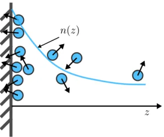
• The active Brownian particle model
• Pressure in active colloids

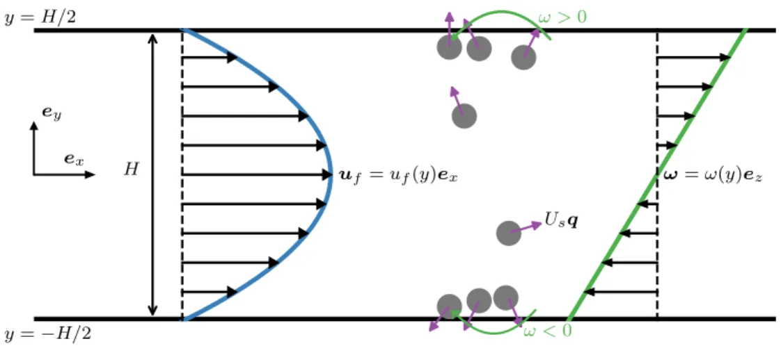
In other words, the instantaneous velocity U =𝑈𝑠q: 𝑈𝑠 is the swimming speed and q is a unit vector in the swimming direction. Therefore, the osmotic pressure at the wall is the sum of the osmotic pressure and the swimming pressure far away in the bulk.

Figure 1.1: Schematic of ABPs on one side of an infinite planar wall ( 𝑧 = 0) and the number density distribution.

Thesis outline

• Transport of active colloids
• Microrheology of active colloids
• Activity-induced propulsion

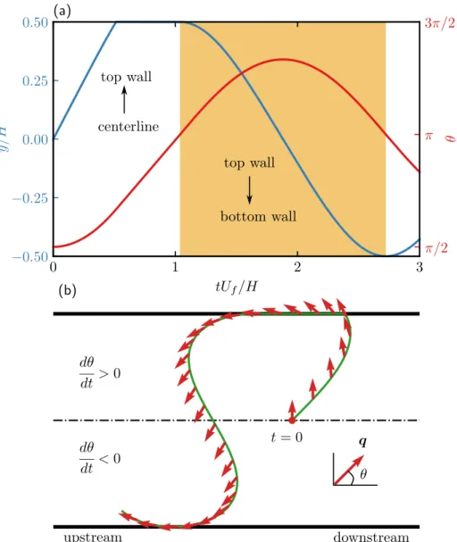
Particles rotate counterclockwise (𝑑𝜃/𝑑 𝑡 >0) in the upper half of the channel and clockwise (𝑑𝜃/𝑑 𝑡 < 0) in the lower half of the channel. When the probe perturbation flow (shown in blue) is included, the density (corresponding to the radial polar order) at the back (𝜃 =±𝜋) becomes higher than that at the front.

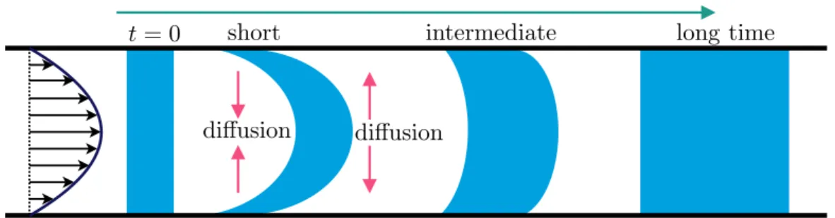
Upstream swimming and Taylor dispersion

Introduction

Matilla et al.(2019) in the context of ABPs in external flow through periodic porous media. The net velocity of ABPs in the longitudinal direction approaches that of passive Brownian particles in the strong flow limit.

Figure 2.1: Schematic of the Taylor dispersion process of passive matter in a pressure driven flow.

Problem formulation

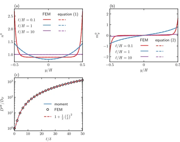
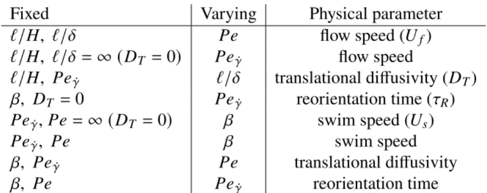
The governing equations are characterized by three dimensionless groups: closing force ℓ/𝐻 = 𝑈𝑠𝜏𝑅/𝐻, activity level ℓ/𝛿 = 𝑈𝑠𝜏𝑅/√. The Péclet number characterizes the relative importance of advection by flow and translational diffusion. We note that the qualitative behavior of the mean displacement and longitudinal distribution does not depend on the dimensionality of the orientation space.

Table 2.1: Variation of different dimensionless parameters and the corresponding physical parameter that is varied.

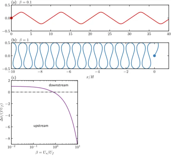
Upstream swimming

• Non-Brownian active particles
• No translational diffusion
• Finite translational and rotational diffusion

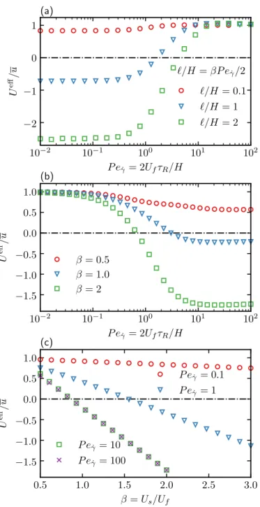
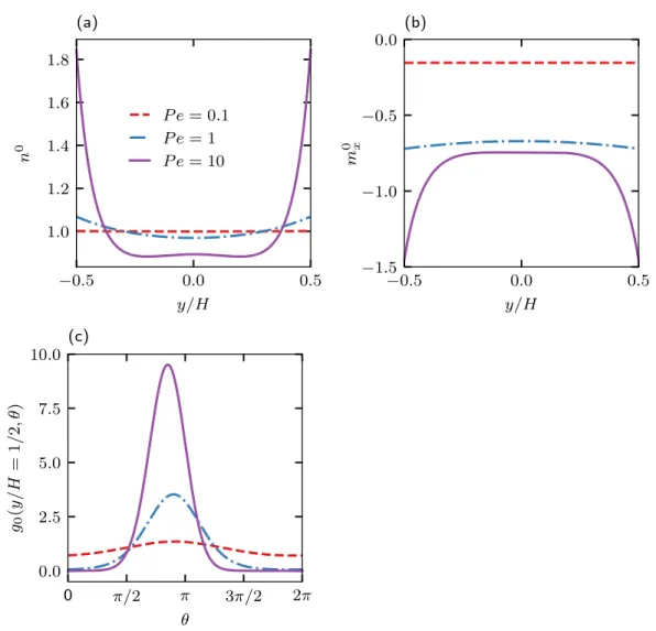
In Figure 2.7(b) we show the average drift 𝑈eff/𝑢 as a function of 𝑃𝑒𝛾¤ for different values ​​of the velocity ratio 𝛽 in the absence of translational diffusion. In Figure 2.8(c), the average field 𝑔0 at the top wall is plotted as a function of the orientation angle 𝜃 for different Péclet numbers.

Figure 2.5: (a)-(b) Trajectories of a non-Brownian active particle for different speed ratios 𝛽 = 𝑈 𝑠 / 𝑈 𝑓

Longitudinal dispersion

• Dispersion in the absence of translational diffusion
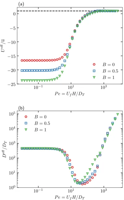
• Dispersion with finite translational diffusion

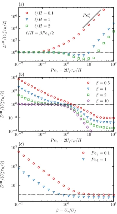
In the classical Taylor dispersion problem, the effective dispersion increases monotonically as a function of the Péclet number. The strong non-monotonic variation of the effective diffusion coefficient as a function of the flow rate (𝑃𝑒𝛾¤) is observed when the translational diffusion is weak (ℓ/𝛿 is large).

Figure 2.12: Variation of the effective longitudinal dispersivity 𝐷 eff /( 𝑈 2

Conclusion

As a result, the spherical ABP model provides a basis for understanding the transport of active particles in channel flow. The effect of the alignment is to improve upstream swimming when the flow is weak.

Appendix: The orientational moments

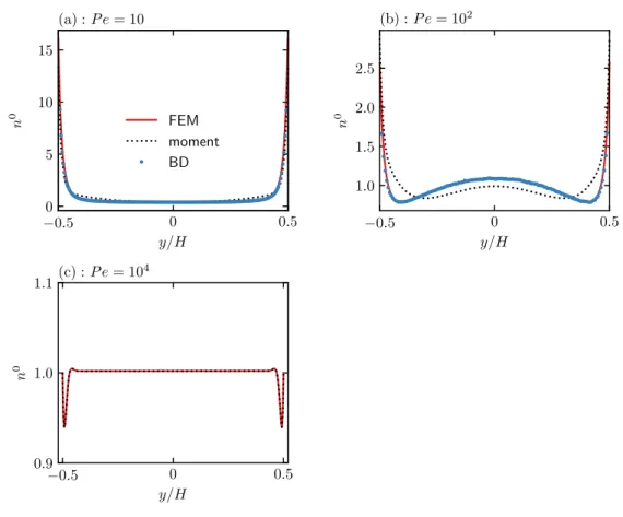
Equation (2.30) together with its boundary condition (2.35) is analytically integrated once to obtain a first-order equation. To solve the average filed moment equations and (2.51), we start from a guess for 𝑛0(−𝐻/2) as a boundary condition and update the guess based on a root finding algorithm so that the normalization condition is satisfied within a tolerance from 10-6.

Appendix: Brownian dynamics simulation

In most simulations, we use a time stepΔ𝑡 =10−3𝑡minku The simulations were run for a duration of 100𝑡maxwu𝑡max is the largest time scale in the problem.

Appendix: Non-spherical particles

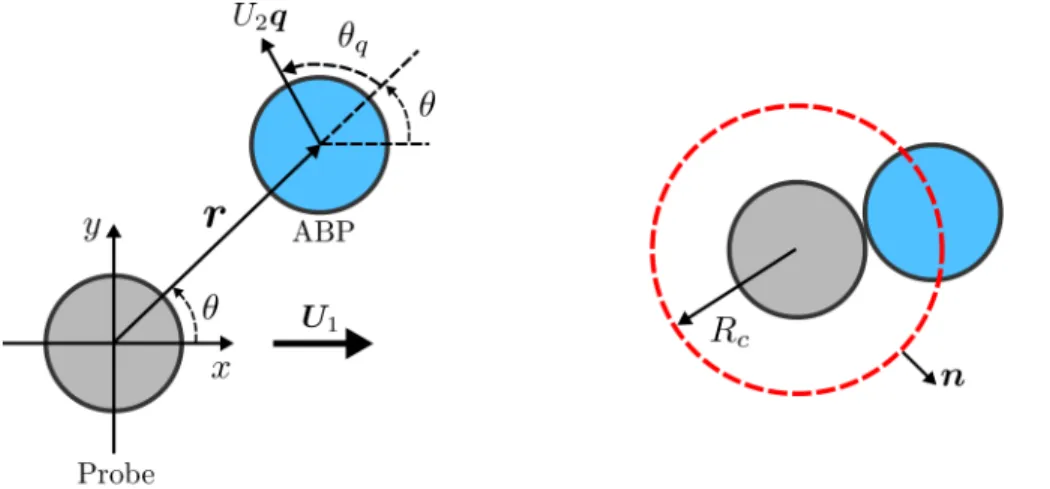
The second dimensionless group is the Péclet number of the probe (using the diffusivity of the ABP). When the probe velocity is zero, that is, 𝑃𝑒 = 0, the microstructure (hence the density) is isotropic, which is simply the distribution of ABPs outside a solid sphere (Yan and Brady 2015b).

Figure 2.15: (a) The average drift 𝑈 eff / 𝑢 as a function of 𝑃𝑒 for different values of 𝐵

Dynamics of an active ellipsoid in a Poiseuille flow

Introduction

Disregarding hydrodynamic interactions between the spheroid and the channel walls, the orientational dynamics of a prolate spheroid in pressure-driven flow is often modeled by Jeffery's equation ( Jeffery 1922 ). Compared to a spherical particle rotating with the local angular velocity of the flow, the spheroid experiences the additional effect of alignment from the stress velocity tensor.

Problem formulation

• Constrained equation of motion in 3D
• Constrained equation of motion in 2D
• Time discretization

In particular, the last term represents the Brownian drift due to the gradient of the mobility tensor. Collisions of the particle with a wall are assumed to be inelastic; the particle and the wall can remain in contact with each other after collisions.

Deterministic dynamics

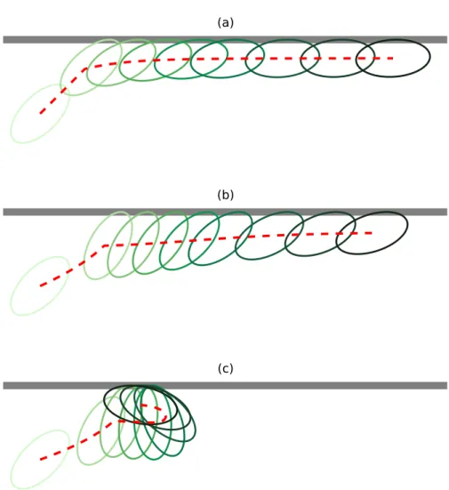
At long times, the particle exhibits a nonzero orientation angle determined by the balance of torque due to flow and contact torque. The ellipsoid then rotates towards the upstream direction and is able to escape into most of the channel.

Figure 3.1: Interaction of an active ellipsoid ( 𝑎 / 𝐻 = 0 . 1 , 𝑎 / 𝑏 = 2) without noise in 2D with the top wall of the channel for (a) no flow, (b) weak flow, and (c) stronger flow

Effective transport

In Figure 3.5, we present the dimensionless effective longitudinal dispersion𝐷eff/𝐷swøm as a function of𝑈𝑓/𝑈𝑠 for different particle shapes. For spherical/point particles, in the small flow limit, the scattering is due to activity and given by the swimming diffusivity𝐷swim =𝑈2.

Appendix: Minimum separation between a spheroid and a planar wall 69

The external vector that is normal to the spheroid surface is in the direction of the vector R𝚲R⊺(y−x). More importantly, the limitation of CF or CV presents a difficulty in meaningfully quantifying probe fluctuations due to a thermodynamic uncertainty bound.

Introduction

In CF mode, the probe is driven by a constant external force Fext and the probe speed fluctuates. For CV mode, the position of the probe is also prescribed and the force fluctuation is infinite.

Mechanics of active Brownian suspensions

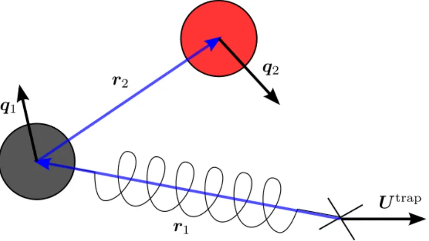
The trap force fluctuations and the position from the trap center satisfy an identical relationship (Wang 2017). Equation (4.2) also implies that we must consider the position rather than the velocity of the probe.

Moving trap microrheology

• Mean and fluctuation of the probe position
• The pair problem
• The probe distribution in the absence of bath particles
• A weak trap
• A strong trap

The average position or average displacement of the probe relative to the trap is defined by. The lowest level problem in the above formulation is the single particle problem of the probe interacting with the trap.

Figure 4.1: Schematic of the pair problem of a spherical probe particle in a moving harmonic trap interacting with a spherical bath particle

Constant-force and constant-velocity microrheology

• Constant-force microrheology
• Force-induced tracer dispersion
• Constant-velocity microrheology

2 = 0 and by integrating out the orientational degrees of freedom of the probe and the bath particle, we obtain the CF microrheology problem of a passive Brownian probe in a passive Brownian suspension. 2 =0 and by integrating the orientational degrees of freedom of both the probe and the bath particles, we recover the equations governing the force-induced spreading of a passive probe in a passive suspension (Zia and Brady 2010).

Fluctuations in a passive suspension

The CV microrheology of an active Brownian suspension governed by (4.80) and (4.81) has been studied by Burkholder and Brady (2020). The pair distribution determined by (4.82) still has high dimensionality even without considering the orientation degrees of freedom, as is the case for a passive probe in a passive suspension.

Derivation of the pair problem

In the dilute limit, we neglect the terms involving the gradients of ln𝑃𝑁−2/2 and use the pair mobility tensor in the absence of other particles instead of ⟨M⟩𝑁−2/2.

Derivation of the variance relations

It can be seen that the net polar order of the probe is not affected by the trap or bath particles. Similar to ⟨q1⟩, the nematic order of the probe regardless of the presence of trap or bath particles is given by.

Asymptotic analysis of the probe in the absence of bath particles

It is clear that in the weak trap limit at this intermediate time scale, the ABP exhibits diffusive behavior with the free space dispersion𝐷𝑇. As long as the trap strength is not identically zero, ABP will eventually (𝑡/𝜏𝑘 ≫ 1) experience the confinement of the trap.

Solution for a passive probe in a passive suspension

A weak density gradient is present in most of the inland areas due to the variation in swimming speed. In the leading order, the probability density in most of the interior is determined by.

Figure 4.2: Definitions of the polar coordinate system and the relative angle 𝛽 = 𝜃 2 − 𝜃 1 .

Constant-velocity microrheology

Introduction

This is done in the dilute limit, where only the interactions between the probe and one of the bath's ABPs matter. For ABPs in the presence of the probe disturbance current, the force thickening originates from the interaction between swimming and the disturbance current.

Figure 5.1: Schematic of a simple shear flow and the force dipoles of a pusher and a puller.

Problem formulation

• The Smoluchowski equation in 2D

Due to the fluctuating nature of the ABP suspension, the external force averaged over Brownian fluctuations is taken into account. Because the bath particles are active, the phase space of the microstructure includes both the relative position r and the orientation q.

Figure 5.3: Schematic of a probe particle driven at a constant velocity U 1 and an active Brownian bath particle in 2D

A slow probe

• Perturbation expansion of the microstructure
• Fast-swimming ABPs
• Zero-forcing microviscosity

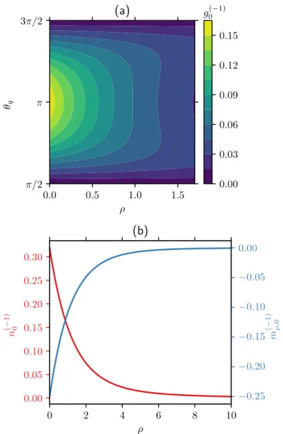
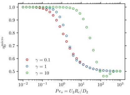
We now consider the suspension microstructure and the zero-force microviscosity in the fast swimming limit characterized by

Figure 5.4: (a): Contour plot of the leading-order distribution function 𝑔 (−1)

Numerical solution of the Smoluchowski equation

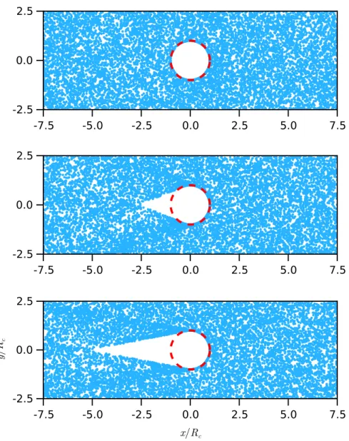
As 𝑃𝑒 increases, a prominently non-uniform density distribution develops at contact with an accumulation at the front and a depletion in the rear of the probe as can be seen in figure 5.8(a). We especially note that the contact density is increased on all sides of the probe.

Figure 5.6: The zero-forcing microviscosity 𝜂 micro

Brownian dynamics simulation

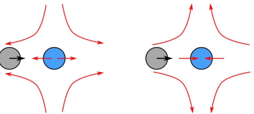
To understand the development of offspring, consider an ABP that is behind the probe (on the left). When the speed of the probe is much larger than that of the ABPs, 𝑈1 ≫ 𝑈2, the trailing wake is quite extended in the horizontal direction.

Figure 5.10: Windowed snapshots of the BD simulation showing the circle of contact (red solid line), the positions of ABPs (blue dots), and the wake structure behind the probe

Microviscosity

Effects of hydrodynamics

• Fluid disturbance due to the active force dipole
• Fluid disturbance due to the probe motion

ABPs in Stokes probe flow experience spatially varying fluid advection and rotate with eddy. For comparison, previously obtained results in the absence of probe disturbance flow are also plotted (see Figure 5.11).

Figure 5.12: Schematic of the flow generated by a pusher (left) and by a puller (right) located in the front of the probe.

Concluding remarks

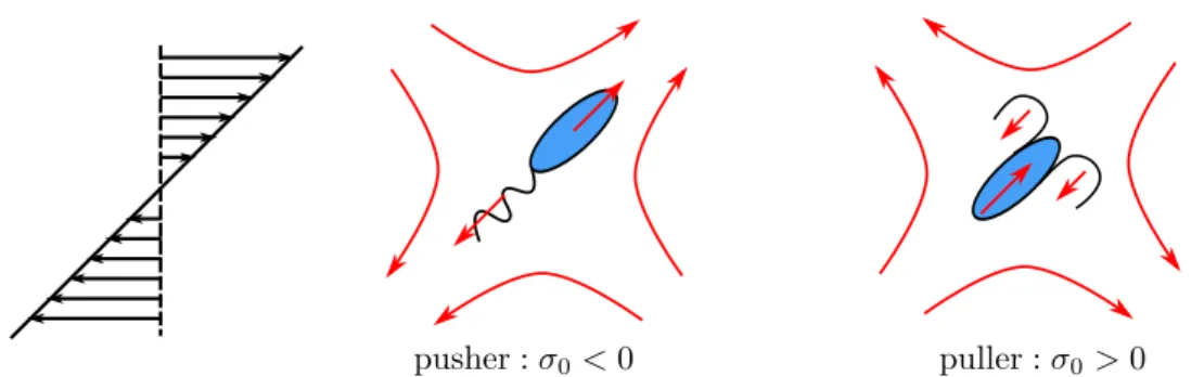
The behavior is reversed in the absence of probe interference, with more ABP pushing anteriorly than posteriorly. In conclusion, we have shown that in the absence of hydrodynamic interactions, the microviscosity of active suspensions is always positive.

Appendix: Orientational moments for a slow probe

It is also important to note that the negative shear viscosity depends on the non-spherical shape of the active particle. This is a manifestation of the so-called linear response where the disturbance fields are proportional to the vector U1 – the weak driving force.

Appendix: The slow-swimming limit

The average density of ABPs inside the vesicle is 𝑛 = 𝑁/𝑉𝑖, where 𝑉𝑖 = 4𝜋(𝑅− ℓ𝑚)3/3 is the volume of the interior. At the inner surface of the vesicle (𝑦 = 0), the leading-order density is large and given by 𝛾2.

Microviscoelasticity

Introduction

In the previous chapter, we studied the microviscous response of active colloidal suspensions. From a theoretical perspective, Khair and Brady (2005) and Swan et al. (2014) discussed the oscillatory microrheology of passive colloidal suspensions.

Theoretical framework

In the absence of hydrodynamic interactions between the probe and the ABP, the translational and rotational fluxes are in the Smoluchowski equation (6.2), respectively. To characterize the microviscoelastic response of the suspension in the dilute limit, a microviscosity can be defined.

Figure 6.1: Schematic of a probe particle oscillating with the velocity U 1 𝑒 𝑖𝜔𝑡 and an active Brownian bath particle in 2D

Small amplitude oscillations

• The governing equations in 2D
• The high-frequency limit

Because the swimming motion is eclipsed by a fast probe, swimming thinning is most important in the slow probe regime and disappears in the fast probe limit. For an oscillating probe, as we consider in this chapter, the swimming motion is likewise obscured in the fast-probe limit and the microviscoelastic response becomes the same as that of passive suspensions.

The zero-forcing microviscoelasticity

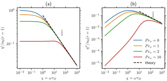
Here, as seen in (6.24), ℎ is driven by the radial advective flux of the 𝑔0 field at contact. In the large𝜒 limit, both the viscous and the elastic part of the microviscosity decay as 𝜒−1/2 [see equation (6.27)].

Appendix: Numerical solution to 𝑓 1 and 𝑓 2

In this limit, the translational velocity of the vesicle is linearly proportional to the driving force - the osmotic pressure. Particles and solvent inside the bubble are treated as a continuum and manipulated.

Figure 6.3: Plot of (a) the viscous part ( 𝜂 ′ ) and (b) the elastic part ( 𝜂 ′′ ) of the zero-forcing microviscosity as a function of the dimensionless oscillation frequency 𝜒 = 𝜔𝜏 𝐷 for several values of 𝑃𝑒 𝑠 = 𝑈 2 𝑅 𝑐 / 𝐷 2

Activity-induced propulsion of a vesicle

Introduction

Of more interest is whether the bubble moves in the same or opposite direction of the concentration gradient. At this high activity limit, ABPs have a thin accumulation boundary layer on the inner surface of the vesicle.

Problem formulation

• The exterior flow
• The interior suspension
• Dynamics of ABPs
• Transport in the membrane
• Dynamics of the vesicle
• Non-dimensional equations for a spherical vesicle

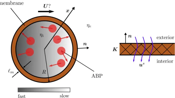
At the inner surface of the vesicle, the flux must vanish relative to the rigid-body motion. Here ℓ𝑚 is the thickness of the membrane and the thin membrane state is ℓ𝑚 ≪ 𝑅 with 𝑅 being the radius of the outer surface.

Figure 7.1: Left: A rigid spherical vesicle with a semipermeable membrane im- im-mersed in an otherwise quiescent viscous fluid

Vesicle motion in the limit of weak interior flow

• Governing equations
• High activity
• A large vesicle
• Vesicle motion due to an external orienting field

This boundary layer structure allows us to relate the osmotic pressure at the inner surface of the vesicle to the swimming pressure outside the boundary layer. The variation of the swimming speed leads to a gradient in the number density in the bulk of the interior.

Figure 7.2: The magnitude of the dimensionless net force on the interior vesicle surface F 𝑤 /(4 𝜋 𝑅 2

Slow variation in activity

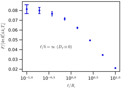
7.4(a), we show the dimensionless net force exerted on the inner wall by the ABPs, F𝑤/(4𝜋 𝑅2 . 𝑖𝑛 𝑘𝑠𝑇𝑠), as a function of the field strength for different values ​​of ℓ/𝑅. For finite thermal diffusion, the net force is reduced and so is the speed of the vesicle.

Concluding remarks

Appendix:Brownian dynamics simulations

Conclusions and outlook

Conclusions

Outlook

The rotational operator

The orientational moments

The spatial moments