For the purpose of this study, we will apply the FTLE-LCS method first proposed by [Haller 2000, Haller 2001], which uses Finite Time Liapunov Exponents (FTLE) to identify Lagrangian Coherent Structures (LCS). The benefit of the FTLE-LCS method lies in the fact that it can be used without hindrance for flows with arbitrary time dependence.
Main contributions of this thesis
The main advantage of the FTLE-LCS method is that it systematically and concisely encodes the Lagrangian data into a single visualization. In light of this result, the LCS move can be thought of as "definitive". the result of a fundamental evolution equation written in terms of the fixed velocity field), rather than 'emergent' (the result of extracting LCS motion from multiple visualization time frames).
Research topics not covered in this thesis
Fast parallelized particle methods for PDEs
Peakons are isolated solutions of a traveling wave that differ from soliton solutions by a discontinuity in their derivative that leads to a sharp peak on the crest of the wave.
Self-Assembly by design
Coordinated Search with under-actuated vehicles
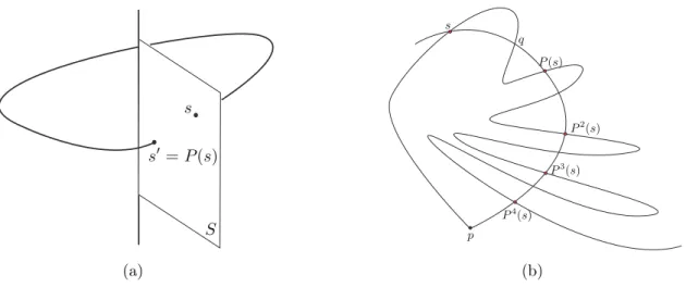
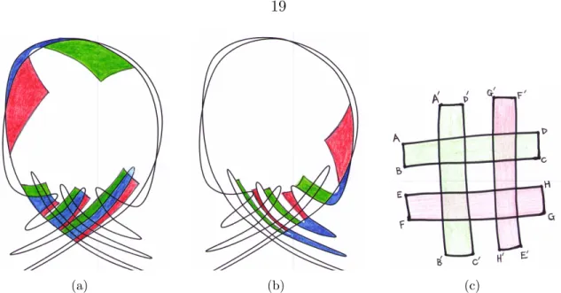
Many of the examples we will encounter in later chapters will be of this form. The intersections and doubling of the back of the manifolds define closed regions in the S-section, called lobes.
Smale and the horseshoe map
Differentiation of the flow map is performed via finite differentiation to yield the FTLE at each point in D . The choice of the integration timeT is therefore also linked to the relevant length scales that are most active in the flow.
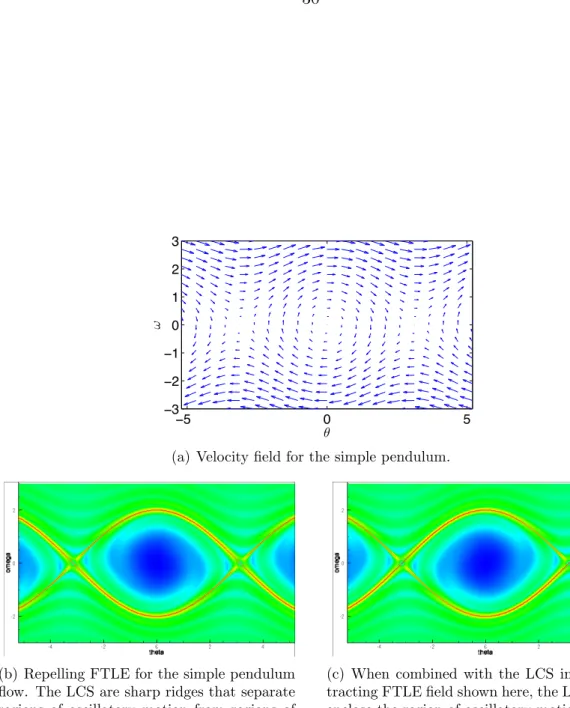
The simple pendulum
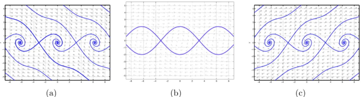
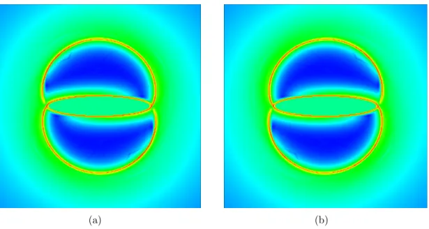
LCS are sharp ridges that separate areas of oscillatory motion from areas of. c) When combined with the LCS in the attracting FTLE field shown here, the LCS completely encloses the region of oscillatory motion.
Monterey Bay
The atmosphere of Titan
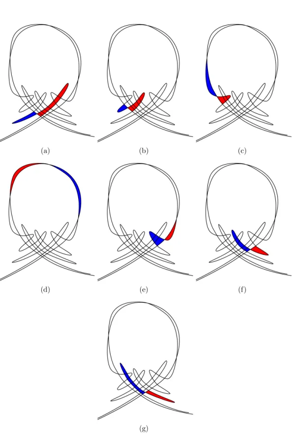
The blue and red drifters located on either side of this divide enter different dynamical regimes: the blue drifters continue to rapidly circle the pole, while the red drifters enter a quiet pocket closer to the equator. In a similar way to the pendulum example, LCS defines a separation between regions with different dynamic results.
Overflows in the North Atlantic
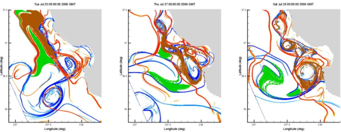
In both cases, the LCS calculation reveals the entanglement structure and its resulting chaotic dynamics in the flow surrounding the vortex. Nevertheless, in the recent IPCC Fourth Assessment Report [Solomon 2007], only one of twenty-four global climate models explicitly simulated mesoscale eddy activity [Bryan 2008]. Near the center of the channel, a north-south ridge is visible on the topography.
As shown in Figure 9-4(a), the ˙x component of the velocity field has a sigmoidal shape in space. as a function of the x-coordinate. To examine the flux across the LCS, we plot the x-location of the LCS. The material line, on the other hand, lags behind in the wake of the current.
Integration of these equations will provide the necessary quantities in the LCS point development formula. Description: FTLE IntTLength is the integration time used in the definition of FTLE.

The elliptic three-body problem
The Kida vortex
The ellipse rotates around its center at a speed proportional to the strength of the vortex. Morton investigated the character of individual Lagrangian trajectories in this flow for different aspect ratios of the ellipse [Morton 1913].
The ellipsoidal vortex
Unforced case
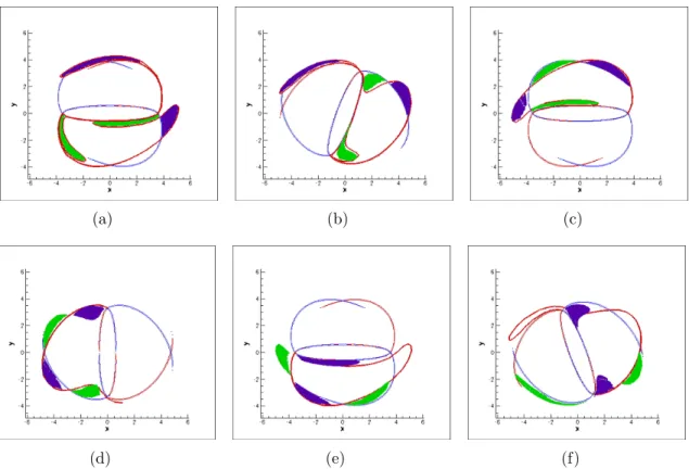
LCS reveals a homoclinic manifold and coincides with stable and unstable manifolds associated with a fixed point at the origin.
Forced case
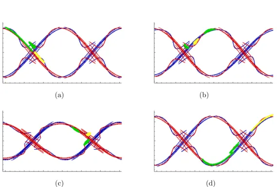
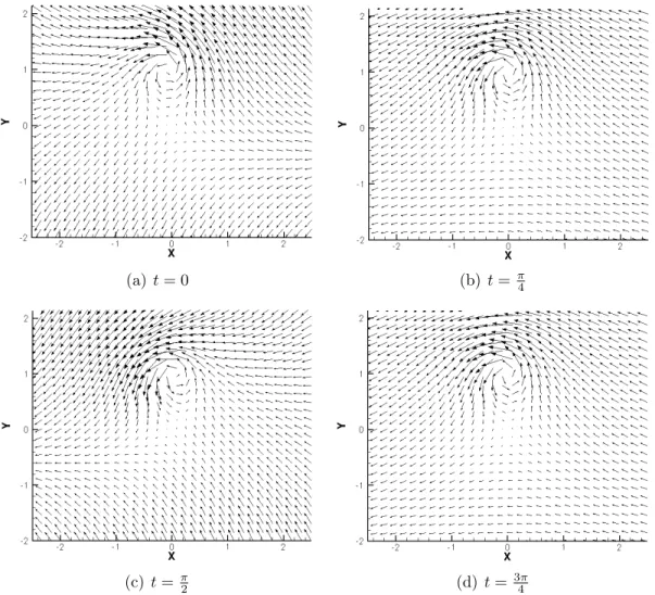
Distinguishing the important transport mechanisms from snapshots of the Eulerian velocity field is not intuitive. Figure 6.3 shows snapshots of the LCS computed for the forced system using an integration time of 10 time units. The lob with blue drifters is taken out of the vortex, while the lob with red drifters is carried into the vortex.
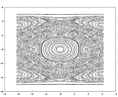
The LCS method shows how the chaotic sea surrounding the resonant region in the Poincar map is formed by repeated stretching, folding and intersection of the lobes.
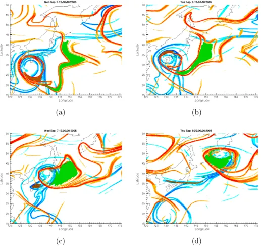
Transport in Typhoon Nabi
LCS reveals that transport into and out of the cyclone is well described by the lobe dynamics. Calculations of the LCS for several typhoons have revealed that mixing via lobes in a homoclinic tangle is a generic dominant feature in tropical storms. We also note that careful examination of the LCS calculated for hurricane flows in fine detail reveals all the intricacies of the homoclinic tangle as studied theoretically in geometric mechanics.
For example, the operation of Smale's horseshoe and the first iteration in the formation of the Cantor set can be clearly seen in the development of the LCS.
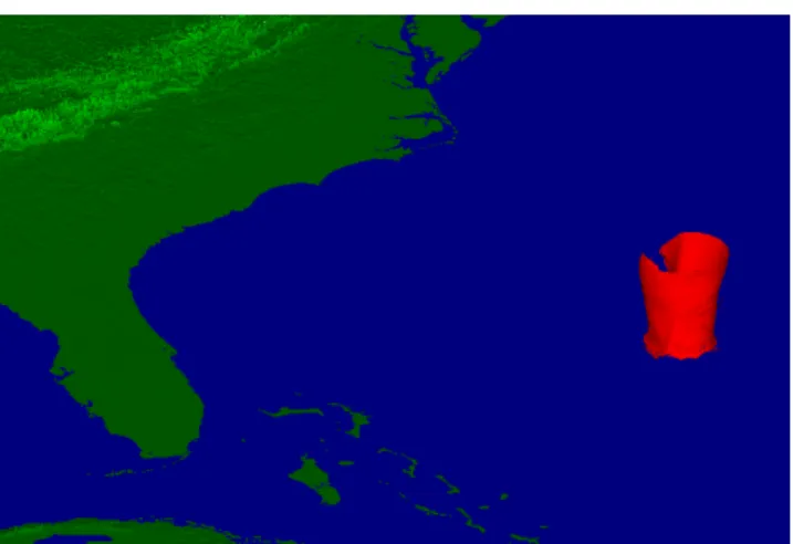
Eye-wall structures in Hurricane Isabel
Meteorologists typically define the eyewall as the locations of maximum wind speed on jets originating from the eye of the storm. Thus, the surface revealed by the LCS is a precise definition of the eyewall corresponding to the Lagrangian dynamics of the flow. The green drifters are initially located in a lobe region that protrudes from the southwest edge of the eye.
This property is revealed by placing passive drifters in the different regions defined by the LCS and observing their trajectories under the action of the flow.
Reanalysis data for the global ocean
The unperturbed case
Here we can immediately conclude that the evolution of the mean amplitude in the unperturbed case is given by the single scalar equation. This degeneracy of the Hamiltonian implies that the system does not satisfy the assumptions of classical KAM theorems and therefore simple KAM theory cannot be applied [Wiggins 2003]. Standard statements of averaging theorems require that all components of the frequency vector α be strictly greater than 0 (see, for example, the statement of the averaging theorem in [Arnold 1978], or the discussion in chapter 8 of [Sanders 2007] about passage through resonance and the absence of theory to handle the fully resonant case).
As such, the reduced equation does not capture important details in the dynamics arising from the inherent non-integrability, and in particular the complex influence of the higher-order components in the mean mode.
Perturbed case
The approach proposed here to obtain a closed equation for the mean amplitude includes the influence of higher order modes by incorporating explicit time dependence in the perturbation term and therefore leads to a one and a half degree of freedom system. The coordinate transformation and subsequent approximation yields a single non-autonomous ordinary differential equation that includes approximate dynamics for the higher-order scales and whose solution approximates the dynamics of the mean angle of the system. In fact, the information contained in the higher order states remains in the lower order description via the initial conditions.
The method just described is now applied to a simple coupled oscillator model for biomolecules, where preserving the influence of higher modes in the dynamics is essential to accurately recover the non-trivial dynamics of the conformational change.
Conformation change in biomolecules
- The model
- Properties of the model
- The reduced order model
- Efficient actuation of conformation change
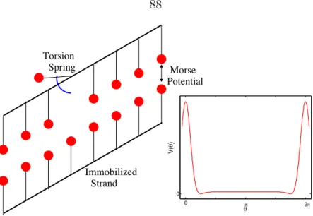
The argument of the Morse potential is the distance between complementary base pairs projected onto the vertical. By definition, we say that a global change in conformation has occurred when the average angle of the pendulum passes through sradians. The amount of energy required for robust spin induction strongly depends on the frequency content of the initial state.
The action of the zipper consists of 31 small strokes (energy = 0.0245), which deliver a total energy of 0.75 to the pendulum chain.
Visualizing transport in the reduced model
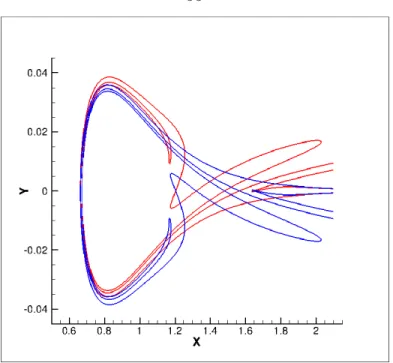
Construct a uniform grid of initial conditions in the mean angle phase space in the reduced model. Before an initial state in the reduced mean-angle phase space can be ascended, it must first be ascended to the full 2N-dimensional phase space. As for the turbulent pendulum of Chapter 4, the intersection of the blue and red boundary surfaces define the lobes that mediate transport in the flow.
For perturbations in higher order modes, the transport structures in the reduced model are visually indistinguishable from those of the full model.
Invariance of the LCS
Motion of a Flux Minimizing Surface
The approach that enables the visualization of the homoclinic tangle in aperiodic flows is the FTLE-LCS method. In addition to the applications, we have addressed some important theoretical foundations of the LCS method. Many of the features available in raw2tec still need to be included in the raw2mat.m script.
Description: Atmos Radius is the radius of the sphere to be used for integration on the sphere. Description: Boundary InFile is the name of the file containing the list of polygon segments to be used for the boundary. Description: Velocity Null[ND] is a switch to turn on/off the nulling of the velocity along the specified dimension.
Equations of Motion for the LCS
MPI
Description: Data Periodic[ND] is a switch to turn data periodicity along the specified spatial dimension on/off. Description: FTLE width is the width of the Gaussian filter that will be used in the smoothing after the FTLE process. Description: Plot OutFile is the name of the file where the plotted velocity output data will be placed.
Description: Track File is the name of the file containing the track coordinates to be used to calculate the FTLE for moving grids.
GSL
Make Newman
A shell script is provided that will attempt to compile Newman in two, three and four dimensions. This will attempt to generate three executables: newman2D, newman3D and newman4D in the ./src folder. If you run into compiler errors, or if you want to customize the installation, you may need to edit the makefiles.
The most common compiler error is making sure the linker can find the necessary libraries.
Running Newman
Viewing the Results
Tecplot Format
Use the -s flag to convert from spherical to Cartesian coordinates for drawing on a sphere. For 3D data on the sphere, use the -a option to give the scale factor by which the atmosphere can be scaled relative to its true size.
Matlab Format
Parameters
Description: Data Res[ND] is the number of grid locations in the numeric speed data. Description: FTLE TrackWidth[ND] is the width of the grid used to calculate the FTLE centered around the storm center when the Track Storm option is used. Description: Nest list is an ordered list that specifies which of the nested rate sets to use for the calculation.
Vulpiani, Predictability in general: an extension of the Lyapun exponent concept, Journal of Physics A: Mathematical and General.