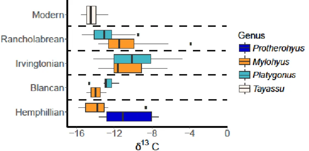
The single line within each box represents the median value, while the upper and lower bounds of the box represent the first and third quartiles, respectively. The single line within each box represents the median value, while the upper and lower bounds of the box represent the first and third quartiles.
Overview
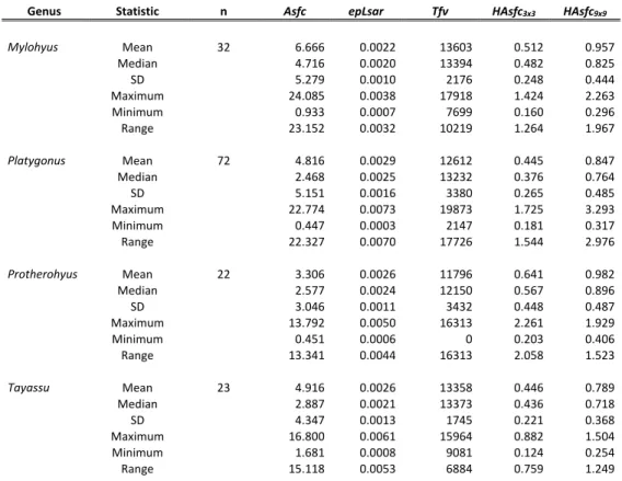
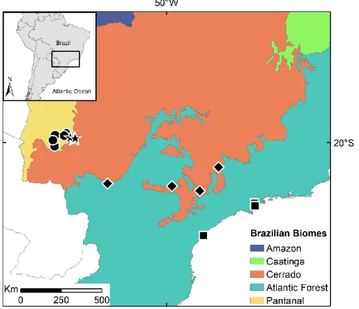
Heterogeneity of complexity (HAsfc) measures the variation between textural features across a surface, while texture fill volume (Tfv) numerically reflects both the shape and texture of the surface, specifically its concavity and convexity (Scott et al., 2006). The land deforested in the Pantanal is largely devoted to livestock farming (Seidl et al. 2001). The semi-deciduous Atlantic Forest is a transitional area between the Atlantic Forest and the Cerrado biome, consisting of sites with flora indicative of the Atlantic Forest biome and sites with flora from the Cerrado biome (Ribeiro et al. 2009).
A complete overview, design concepts and details (Grimm et al. 2010) for the model can be found in the supplementary material. The maximum stride length was selected from the GPS movement data and is the greatest distance traveled in a three-hour period by any of the white-lipped peccaries studied (Jorge et al. 2019). On the other hand, Morante-Filho et al. 2015) concluded that less than 50% forest cover reduced species richness for tropical birds.
Therefore, pathways that maintain tropical forests while informing landscape planning are essential (Lewis et al. 2015). Between 2013 and 2015, 12 white-lipped peccaries were captured and fitted with GPS collars in the southern Cerrado in central Brazil (Jorge et al. 2019). Emergence – The spatial orientation and distribution of habitat use intensity (measured in the model as visitation frequency) emerges as a function of the specified percentage of forest cover, the number of forest fragments in the landscape and the distance between fragments.
Organization
Introduction
Hurtado etc. 2016), understanding tayassuid ecology both today and in the past can provide information on how dietary preferences have changed both over time and in response to past climatic fluctuations. However, they have also been documented to consume additional leaves in times of food scarcity (Sowls 1984; Keuroghlian et al. 2009).
Background
- Evolutionary history of the tayassuidae
- Paleoecology of extinct peccaries
- Ecology of extant peccaries
- Dental Microwear Texture Analysis (DMTA)
- Geochemical data
In addition, Tayassu consumes a greater variety of fruits during the rainy season when more fruits are available (Keuroghlian et al. 2009). Values between these two endmembers reflect mixed feeding diets in extinct taxa (Cerling et al., 1997; Cerling and Harris, 1999; Kohn, 2010).
Materials and Methods
- Sample Collection
- DMTA
- Geochemical Analysis
- Statistical Methods
When comparing with modern taxa, an additional 1.5‰ is subtracted from each stable carbon isotope value for extinct specimens to account for increased CO2 emissions since the Industrial Revolution, the Suess effect (Cerling et al. 1997; Cerling & Harris 1999; Passey et al. al. 2005). Stable carbon isotope values below – 9 ‰ indicate a diet primarily composed of C3 plant material, while values greater than – 2 ‰ indicate a diet primarily composed of C4 plants, in extinct peccaries (Cerling et al. 1997; Kohn 2010).
Results
DMTA
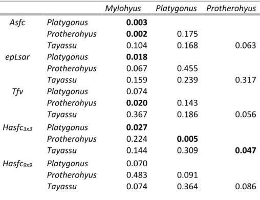
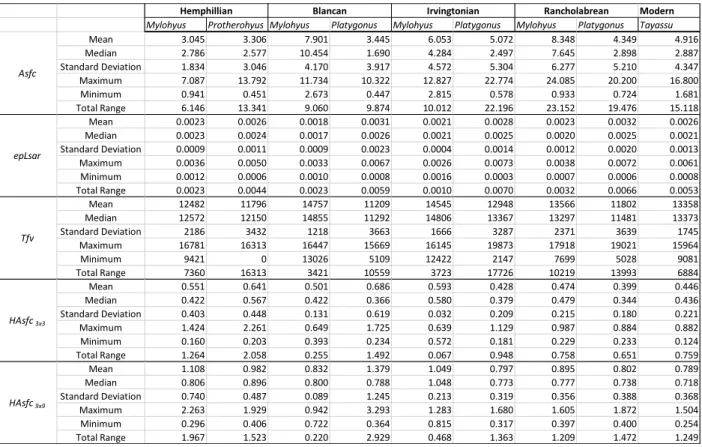
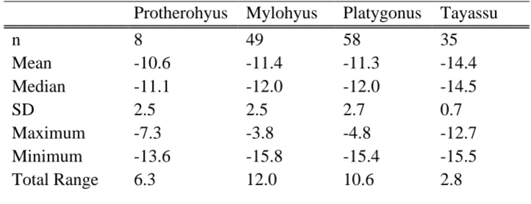
Asfc, area-scale fractal complexity; epLsar, anisotropy; Tfv, texture fill volume; HAsfc3x3, HAsfc9x9, Heterogeneity of complexity in a 3 x 3 and 9 x 9 grid, respectively; SD, standard deviation (n – 1); Extent, total extent of all samples examined. Asfc, area-scale fractal complexity; epLsar, anisotropy; Tfv, texture fill volume; HAsfc3x3, HAsfc9x9, Heterogeneity of complexity in a 3 x 3 and 9 x 9 grid respectively; SD, standard deviation (n – 1).
Stable carbon isotopes
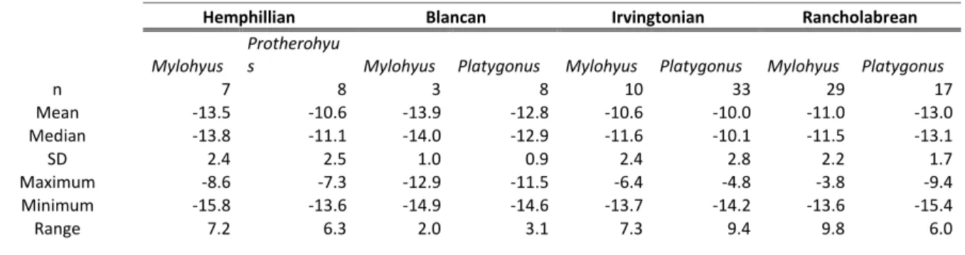
However, Mylohyus stable carbon isotope values during the Rancholabrean and the Irvingtonian do not differ from each other, nor do they differ between the Hemphillian and the Blancan (Table S8). All stable carbon values for extinct genera have been adjusted by –1.5 ‰ to account for increased emissions since the industrial revolution (Cerling et al., 1997; Cerling and Harris, 1999; Passey et al., 2005).
Discussion
Extinct Peccaries
The environment during the Irvingtonian may have been more open than the early or later Pleistocene, as indicated by the higher δ13C values from Platygonus and Mylohyus during this time period, and previous studies (DeSantis et al., 2009). All mean tayassuid isotope values are below –9 ‰ suggesting that none of the peccaries in this study had a predominantly C4 grazing diet; however, the higher isotopic values indicate that at least some C4 sources were consumed by Platygonus and Mylohyus. Further, Mylohyus was not restricted to the forest in terms of food consumption during the Irvingtonian and Rancholabrean NALMAs, as δ13C values are representative of a broader diet including C3 and C4 sources during these time periods.
Mylohyus is eating C3 and C4 food sources, the δ13C values for Platygonus are consistent with those of a predominantly C3 browser. The transition from lower δ13C values in the Hemphillian and Blancan to higher values in the Irvingtonian is consistent with previous studies documenting that some Irvingtonian sites occurred during interglacial periods and were.
Modern peccaries
Perhaps the ability to change diet was not a sufficient survival mechanism for tayassuids and.
Conclusions
Introduction
Beck 2005; Keuroghlian and Eaton 2008a, 2008b; Desbiez et al. 2009), stable isotopes can often reflect a much broader picture of diet, including seasonal variations in diet, relative trophic position or environmental and habitat preferences (van der Merwe &. Stable carbon isotopes (δ13C) from mammalian hair can determine whether an organism's diet consisted of predominantly by plants using the C4 photosynthetic pathway or those using a C3 pathway (Bender 1971; Sponheimer et al. Examples of common C4 plants include warm season grasses, sugarcane and maize (Ehleringer & Bjorkman 1977; Klink & Joly 1989; et al. 1999).
Isotopically, C4 plants will have higher δ13C values than C3 plants, as the C3 photosynthetic pathway discriminates to a greater extent against the heavy 13C isotope (Bender 1971; Ehleringer et al. 1991). This phenomenon occurs due to discrimination against the lighter 14N isotope during shedding (e.g., Loudon et al. 2007; Ben-David and Flaherty 2012).
Materials and Methods
Field Sites
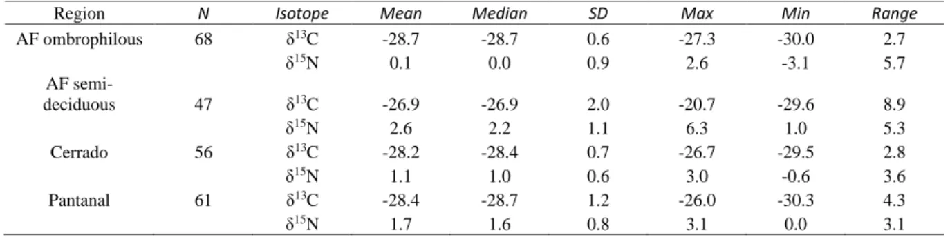
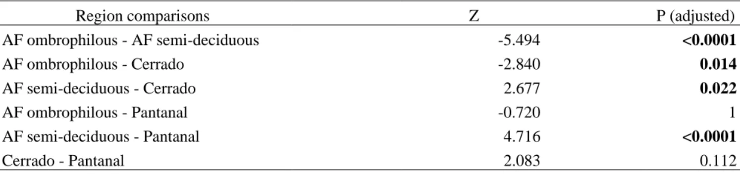
All samples collected from the Atlantic semi-deciduous forest were collected directly from sites containing Atlantic Forest flora. Sources from the Atlantic semi-deciduous forest did not differ in δ15N compared to other regions. The distribution of stable nitrogen isotopes was not different between hairs and springs in the Atlantic semi-deciduous forest.
The samples from the Atlantic semi-deciduous forest allowed a comparison at two time levels, before 2000 and 2016. The main crops grown in the Atlantic semi-deciduous forest are soybeans, sugarcane and maize.
Introduction
LINKING AREA-BASED MODELING AND ANIMAL MOVEMENTS TO ASSESS CHANGES IN HABITAT USE BY MOBILE FOREST-WINGING SPECIES I. Here we propose a new way to determine fragmentation thresholds using animal movements and habitat use patterns. We created a spatially explicit agent-based model to assess how the amount of forest cover and the spatial orientation of forest fragments affect animal habitat use patterns and therefore.
Furthermore, our model allows an evaluation of how habitat use patterns are altered in fragmentation environments that are not necessarily testable in field studies. We investigate under which spatial conditions changes in landscape configurations alter animal habitat use patterns and evaluate whether habitat use patterns change gradually with fragmentation or whether thresholds exist at which habitat patterns change dramatically.
Methods
Model Purpose
White-lipped peccaries are forest-dwelling ecosystem engineers that are not functionally redundant (Keuroghlian & Eaton 2008a; Beck et al. 2010; Jorge et al. 2019). They directly affect the ecosystems where they are present by creating habitats for other organisms (Keuroghlian &. Areas where white-lipped bakers have become locally extinct have caused dramatic changes in forest structure and loss of biodiversity (Silman et al.
Model Description
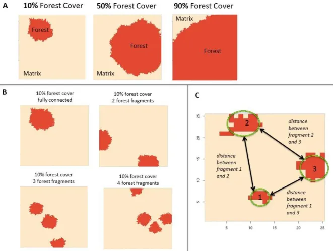
The loss scenario is determined by the percentage of forest cover and the fragmentation scenario is determined by the number of forest fragments (Figure 7A-B), as studies have. When the number of forest fragments is set to one, the forested cells form a single unit, or a single forest fragment (eg, Figure 7B). However, in simulations with a larger number of fragments, habitat use patterns reflect percent forest cover, number of forest fragments, and distance between forest fragments.
Each combination of percent forest cover and number of forest fragments (40 in total) was replicated 30 times, comprising a total of 1,200 landscapes and simulation runs. Despite specifying a specific percentage of forest cover and number of forest fragments combination for each of the 30 iterations, none of the 30 iterations were accurate.
Results
- Two-fragment scenario
- Three-fragment scenario
- Four-fragment scenario
- All fragment scenarios
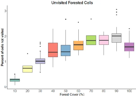
Between 60% and 40% of forest cover, a greater number of simulations led to scenarios where a greater number of forested cells were not used at all (Figure 10A). For each habitat loss scenario, the number of simulations resulting in 1, 2 or 3 forest fragments on the landscape;. For each habitat loss scenario, the number of simulations resulting in 1, 2, 3 or 4 forest fragments on the landscape;.
Between 70% and 60% forest cover, an increased number of simulations resulted in scenarios that did not use a larger number of forested cells ( Figure 12A ). With the increased number of forest particles, more forest cover was needed before bakers could use all the landscape particles.
Discussion
Therefore, at this forest cover threshold, habitat use patterns mimicked those seen in the one-fragment simulations. At 50% forest cover and below, there is a qualitative change in forest habitat use patterns, resulting in a large variation in the number of forested cells that were not used (Figure 12A). Regardless of fragmentation level, at or above 70% forest cover, peccaries used all fragments of the landscape (Table 12, Table 14-15, Figure 10-12).
Our model results did not support a sustainable landscape with only 10% forest cover, regardless of the spatial orientation of the forest fragments, unless those fragments were fully connected. Yet others have suggested that a minimum of 50% forest cover is essential to maintain species richness and abundance of forest specialist seed dispersers (Morante-Filho et al. 2015; Melito et al. 2018).
Conclusion
In addition, it should be noted that when applying the model results to conservation decisions, it is important to consider scale (Fahrig 1998), such as the minimum amount of forest cover needed to sustain a population. Here we did not specify a minimum fragment size to sustain populations, rather we investigated how the fragment size would affect habitat use patterns if peccaries could survive in a patch of that size. Nevertheless, the fragment size in our model needs to be scaled up to reflect the minimum fragment size necessary for peccary populations to sustain (see Jorge et al.
Synthesis
Outlook
Dietary ecology of the extinct cave bear: evidence of omnivory as inferred from dental microwear textures. This model is programmed in R version 3.3 and the version of the model used therein. Because the rate parameter of the associated exponential distribution varied across peccaries, we used the median value for use in the model.
Additional details of each of the actions performed here can be found in the Submodels section. After choosing the step length and the direction to travel in, the model finds the coordinates of the end point. If the endpoint of the selected path is off the grid, the agent selects a new stride length and turn angle.
Cross matrix or stay – If the endpoint of the set path lies within an isolated forest.