In the first part, we will relate the analytical structure of the scattering amplitudes of scalar quantum field theories in the far infrared to unifying symmetries of their actions in the ultraviolet. In Chapter 3 we review the Hamiltonian formulation of binary dynamics and outline the extraction of the effective Hamiltonian from scattering amplitudes.
Introduction
The final and strongest assumption is a variation of Adler's null condition [9,10], in which we demand that all tree-level amplitudes vanish when a massless degree of freedom is softened. Interestingly, we find that our four criteria imply that the side space of the symmetry break is symmetric.
Perturbative Unitarity
To avoid this annoyance, we manifest high-energy scaling at the level of the Lagrangian by defining a 'minimum operator basis', analogous to the minimum kinematic basis for amplitudes. To derive an analog of the minimum kinematic basis for amplitudes in Eq. 1.1), we use integration in parts to shuffle all derivatives acting on 𝜙𝐼.
Soft Theorems and Unification
Under the affine symmetry defined in Eq. 1.26) means that the components of the vector 𝜆𝐼 are different from zero only if 𝑚𝐼 =0. This is expected because X =(𝑋𝐼 𝐽, 𝜆𝐼) is a generator of the coset space𝐺/𝐻and is thus defined only modulo the addition of the generator T = (𝑇𝐼 𝐽,0) of the continuous group𝐻.
Linear Sigma Model Example
For the first case, the pion 𝜋𝑖 is a free massless scalar decoupled from the rest of the theory. We can also see that the Lagrangian is equivalent to that of the linear sigma model by defining a multiple of fieldsΦ𝐼 = (𝜋𝑖, 𝑣+𝜎), so Eq.
Conclusions
In the gauge-invariant observational approach [58], the radial action is related to the logarithm of the conservative amplitude by Eq. We will now present the first calculation of the radiated angular momentum in the extended KMOC framework.
Gravitational Binary Dynamics
Introduction to Gravitational Binary Dynamics
The first complication, scattering through the radiation reaction force, is the focus of the present work. However, these times are simple functions of the distances between the charges and the speed of light. Transformations with respect to 𝒓,
In the classical case of a non-relativistic binary system interacting through a conservative force that depends only on the relative displacement, the COM transformation trivializes the dynamics of the center of momentum. As it turns out, the "mixing" of the COM and relative degrees of freedom in the arguments of the forces does not appear at𝐺3order Through𝐺3order, then, the equations of motion for the binary system uncouple5,.
Conservative Binary Dynamics
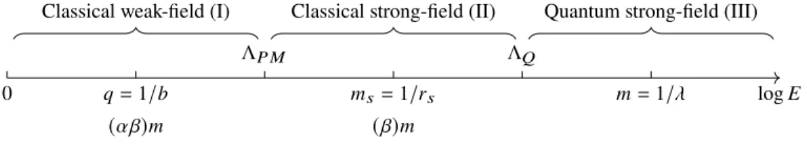
Determine which amplitude topologies (off-shell diagrams or on-shell cuts) contribute to the gauge invariant quantity in the classical limit, and discard all others. In quantum theory, the extra distance scale that poses the problem is the Compton wavelength associated with the total binary mass, 𝜆 = ℏ/𝑚. Since fully quantum amplitudes exist on both sides of the comparison equation, both yield superclassical terms in the semiclassical limit.
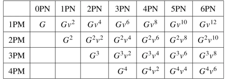
Orders 𝛼𝑝 <ℓ−2 will have negative powers of 𝛽 in the observable, and are therefore superclassical. To summarize, classical𝑛PM (𝐺𝑛) contributions to the observable come exclusively from (ℓ =𝑛−1) loop diagrams in the amplitude.
Dissipative Binary Dynamics
Returning to the expectation expression Eq. 4.8), we expand𝑆=1+𝑖𝑇, where the operator𝑇 describes the non-trivial part of the distribution. Remembering that the unitarity of 𝑆 implies. 4.13) to eliminate 𝑇† in the first term of the right-hand side of Eq. This leads us to the construction of ansätze for energy and angular momentum fluxes.
Working in the Hamiltonian formalism, we conclude that the gauge transformations of the full theory induce canonical transformations of the binary phase space (𝒓,𝑹, 𝒑,𝑷). 𝐽 captures a total force of the angular momentum of the initial scattering plane 𝐽 which is also present in the fluxesF𝐽.
Radiated Angular Momentum from Scattering Amplitudes
Observables, Symmetries, and Form Factors
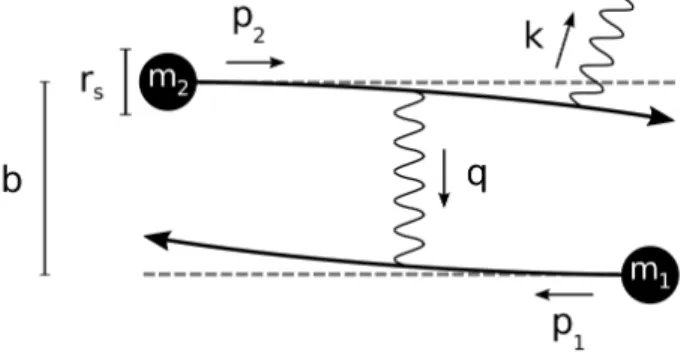
We are interested in the total linear and angular momentum radiated in the form of electromagnetic and/or gravitational waves in the process, which we denote by Δ𝑃𝜇1 and Δ𝐽𝜇 𝜈 respectively. Note that we only need to consider the combination 𝑢𝑖· (𝑏1+𝑏2) because in the classical limit 𝑏𝑖 is orthogonal to 𝑢𝑖, i.e. of the radiated momentum and angular momentum2.
As we will see, our choice manifests the fact that the observables are polynomials in measures. All form factors are functions of mass only,
Linear and Angular Momenta in the KMOC Framework
59 This expression transforms under the action of the Poincaré group on the Fock space as. The derivation of the differential operator in the case of angular momentum is considerably more complicated, so we will only present the results here. In the KMOC framework, the momentum-space wavefunctions 𝜙𝑖(𝑝𝑖) are chosen to describe massive particles in the classical limit and thus peak around the classical momenta 𝑝cl. 4.14) can be calculated in terms of momentum eigenstates|𝑝𝑖⟩ using the definition of 'i' states in Eq.
As explained in [42], any momentum transfer 𝑞𝑖 is considered to be O(ℏ) if we take the classical limit.) We can define a radiant core as follows. 4.35) When 𝑋 is empty, for the leading order in the 𝑞 expansion it simply becomes the Fourier transform of the amplitude. We finally arrive at a simple equation for the change of the classical observableΔ𝑂 in terms of the radiation nucleiR.
Scattering Amplitudes
As before, O is defined by O in terms of some formal manipulations that are explained below for the specific examples under consideration. Within the classical localization, the moments 𝑝𝑖 are not yet localized to their classical values and differ by deviations of order O (𝑞𝑖). For this reason, at the beginning, these 𝑝𝑖, unlike classical moments, are not yet orthogonal to the influence parameters 𝑏𝑖.
Only at the very end of the calculation, when all (differential) operators work, can we set all moments to classical values that satisfy the expected orthogonality conditions.
Classical Observables from Scattering Amplitudes
4.62) Given the exponential form of the soft S-matrix, it is easy to calculate its contribution to angular momentum, for spin mediators. Adding everything together, we write the contribution of the soft graviton (the case of 𝑠=2) to the angular momentum as . We now consider the finite energy graviton contributions to the radiated angular momentum in Eq.
With the help of the corrected operator in Eq. 4.84), we can now calculate the coupled dynamical contribution to the radiated angular momentum from Eq. 4.47), which involves a second dynamic radiation core. In contrast to the radiated momentum kernel, the radiated angular momentum kernel is only defined up to a surface term of the form.
Results
As we shall see, there is more to the residual gauge dependence of fluxes than induced canonical transformations. To understand the transformation properties of instantaneous fluxes F𝐸/𝐽, we need to be more precise about their definition in the full theory. The flux gauge transformation thus includes the active canonical transformation (in the sense of 𝜒)Φ:F𝑄(𝜒) ↦→ F𝑄 ◦Φ−1(𝜒).
As with the Hamiltonian/Kamiltonian transformation, both the function and the point at which it is evaluated have changed. In the language of the method of regions, we are interested in regions where some loop moments are located.
Instantaneous Fluxes and the Radiation Reaction Force
Energy and Angular Momentum Fluxes from Radiated Charges
This part of the calculation is analogous to the extraction of the Hamiltonian from the radial action discussed in Section 3.2. In contrast, the coefficients ¯𝑃𝑛 of the 𝑝2 expansion in (5.10) are only functions of the asymptotic momentum square ¯𝑝2 = 𝑝2∞. 𝐸 should depend on the instantaneous momentum 𝒑(𝑟) as in the expansion of the Hamiltonian (5.9) or the asymptotic momentum 𝒑¯ as in the expansion of the momentum squared variable (5.10).
By consulting equation (5.8) and noting that the PM expansion of the total radiated energy Δ𝐸 begins at 𝐺3 order, it is clear that we only need expressions for𝑝𝑟 and𝜕 𝐻/𝜕 𝑝2to leading (𝐺0) order to calculate F(3). Then why isn't there a dash over the total radiated chargeΔ𝑄 shown on the left side of the matching equation.
Relative Radiation Reaction Force at 3PM Order
We cannot simply perform a gauge transformation of the fields because they were "integrated" in the transition to the effective theory. By assumption, transformations of the whole scale do not change the behavior of the whole system according to Eq. We hinted that gauge transformations of fluxes are more complicated than scalars or Hamiltonians.
In fact, the remaining gauge transformations of flows cannot be described by canonical transformations alone. To ensure that the overlap integral vanishes, however, it is generally necessary to decompose into as many regions as there are poles of the mass scale in the denominator of the integrand.
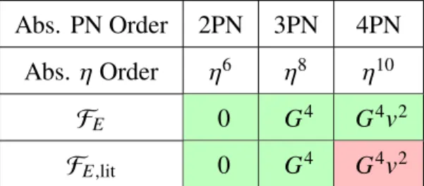
Comparison of 3PM Fluxes to PN Literature
Induced Canonical Transformations
Recall that we calculated each flux by constructing an ansatz and fitting it, term by term, to the PM expansion of the corresponding radiative loss. We then equate the result, term by term, to (the PN expansion of) the isotropic gauge Hamiltonian and use the resulting system of equations to solve for the ansatz coefficients. Thus, the overall power (and hence the PN order) of the Poisson bracket set in Eq. 6.6) increases strictly with the power of 𝜖.
When performing the transformation, we simply determine the lowest 𝐾 such that the 𝑂(𝐾+1) corrections to the truncated transform will be higher order in 𝜂 than the PN expansions we are comparing. The exact value of 𝐾 will depend on the leading PN order of the generator, but such a 𝐾 always exists.
Induced Gauge Transformations of the Instantaneous Fluxes
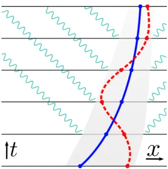
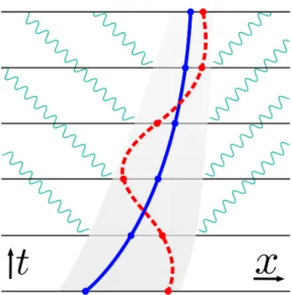
However, a specific choice for the Cauchy surface at one time 𝑡 can be extended to a foliation of spacetime1 by the flow of a time-like vector field, so it is sensible to speak of the instantaneous fluxF𝑄(𝑡) as a function of all 𝑡 ∈ R. The various Cauchy foliations are generally linked by diffeomorphisms of gravitational theory, and so the associated ambiguity in the instantaneous fluxes as functions of time can be taken as a manifestation of gravitational freedom. Thus, the fluxes defined in Chapter 5 as phase-space functions2 of the effective theory have two residual dependencies on the diffeomorphisms of the full theory.
The diffeomorphism connecting the surfaces of Figure 6-2 to those of Figure 6-2 is simply a global shift in the. In this section we will directly compare our phase space expressions with corresponding expressions in the literature, without any need for trajectories.
Schott Terms, Flux Balance, and Small Diffeomorphisms
This constraint can be derived by the leading-order 𝑟 scale in the integrand of Eq. We begin by solving only the coefficient equations of the leading PN order terms appearing in the corresponding equations in terms of the leading PN order coefficients of the ansätze. Let us look again at the erroneous attempt to expand the integrand in the quantum region without taking a cutoff from Eq.
The interesting thing about this dim-reg calculation is that the IR divergence from the quantum expansion of the integrand in the classical region and the UV divergence from the classical expansion of the integrand in the quantum region exactly cancel out. The calculation of the instantaneous power flow coefficient of 4PM requires only a slight change from the asymptotic calculation performed in the previous section.