The marginal utility of a given number of units is the total utility for that quantity minus the total utility for one less unit. Decreasing marginal utility (assuming MU is positive) implies increasing total utility, but at a decreasing rate.
Law of Equi Marginal Utility
For the second unit, the consumer compares the weighted marginal utility of second unit of X and FIRST unit of Y. Continuing in the same way, we learn that the consumer chooses to buy 4 units of X and 2 units of Y.
Indifference Analysis
In this diagram, combination A and B are on the same indifference curve, so they should provide the same utility to the consumer. Similarly, A and C are also on the same indifference curve, so they should also provide the same utility to the consumer.
Multiple Choice Questions (Section 1)
8 The diagram shows the marginal utility that an individual derives from a good at different levels of consumption. 14 The diagram shows the marginal utility (MU) that an individual derives from a good at different levels of consumption.
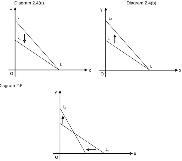
Shifts In Budget Line
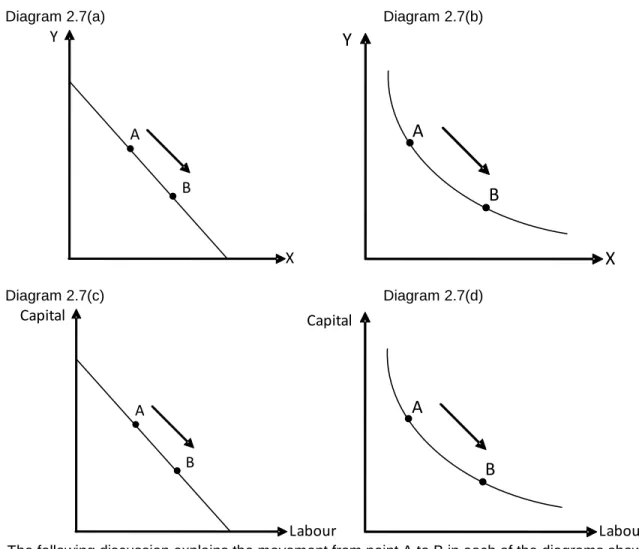
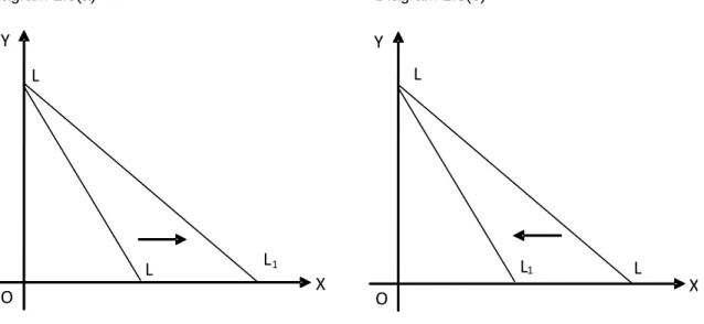
A change in the price of X: A decrease in the price of X (while keeping money income and the price of Y unchanged) decreases the slope of the budget line. A relative increase in the cost of capital (perhaps due to increased interest rates or the removal of the capital subsidy) could also encourage firms to hire more labor relative to capital (try N/02/3/03 & J/02/ 3/05).
Multiple Choice Questions (Section 2)
Assuming there is no change in the price of X, what could explain a shift in the consumer budget line to GH? Assuming there is no change in the price of Y, what could explain a shift in the consumer budget line to GH?
Section: 3 Normal, Inferior and Giffen Goods
Real Income and Substitution Effects of a Price Change
Negative substitution effect and positive real income effect reinforce each other, resulting in a negative price effect. For Giffen goods, income effect is not only negative but also stronger than the substitution effect.
Consumer's Equilibrium
The increased income shifts the budget line toward xx2 and the new consumer's equilibrium will be between points III and IV, as the consumer chooses to move up the indifference curve because of the increased income and purchasing power. However, if the consumer perceives Y as a normal good and X as inferior, the new consumer's equilibrium will be between points I and IV, indicating a decreased demand for X and an increased demand for Y.
Income Consumption Curve (ICC)
Impacts of Changes in Price
If the income effect is smaller than the substitution effect, the new balance will be between II and III. In the event that the effect of negative income is stronger and prevails over the substitution effect, the new balance will be between III and IV.
Multiple Choice Questions (Section 3)
Costs, on the other hand, can be divided into short-term and long-term costs based on time. Labour, on the other hand, is considered a variable input as its quantity can be varied according to the firm's requirements.
Laws of Variable Proportion
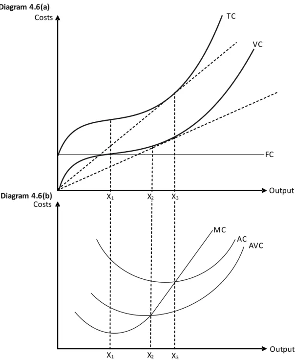
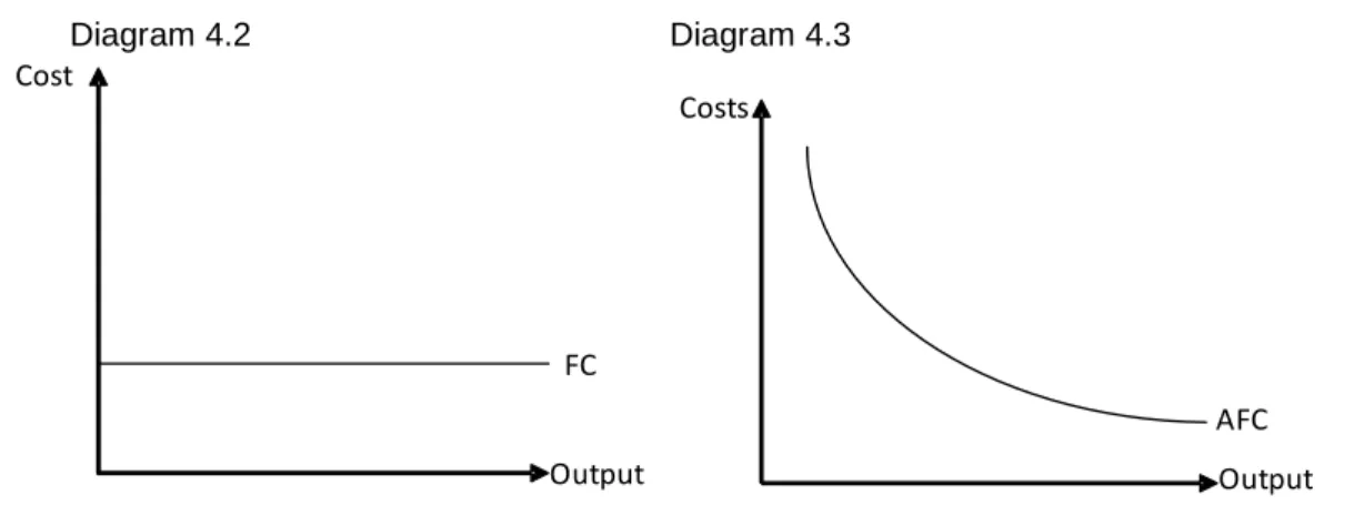
In the short run, total costs can be divided into two categories: fixed costs and variable costs. Total cost and variable cost are parallel curves, the constant difference between them measures fixed cost.
AC AVC MC
Assuming no fixed costs, average cost, average variable cost, and marginal cost are equal and constant for a linear total cost function. Marginal cost is equal to average variable cost, and both are constant for a linear total cost curve (assuming fixed cost equals zero).
Multiple Choice Questions (Section 4)
4. Which explanation explains why short-run labor is subject to the law of diminishing returns. B A reduction in the quality of the variable factor will ultimately result in an increase in production costs. 16 Which explanation explains why labor is subject to the law of diminishing returns in the short run.
Economies of Scale
Opposing economies are economies of scale: increases in unit costs due to the larger size/scale of the firm. External economies of scale are reductions in unit costs due to the size of the industry and/or the location of the company. External economies of scale arise when unit costs begin to increase due to factors beyond the company's control.
Least Cost Combination
Isoquant and Isocost Approach
SRAC 3 SRAC 4
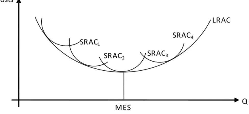
Suppose the firm owns one factory whose short-run average cost curve is SRAC1. It continues to exploit economies of scale until control and coordination problems arise and it reaches a higher average cost curve, SRAC4. Long-run average cost curve is also known as the envelope curve as it touches and encloses all short-run average cost curves.
Minimum Efficient Scale (MES)
The company can increase production only by setting up another plant in the long run with SRAC2 lower than SRAC1 due to economies of scale.
Minimum Efficient Scale (MES) And The Size Of Firms
Natural Monopoly
In the case of a natural monopoly, charging a price equal to MC means lower than average cost. An industry consists of few large enterprises where MES is high and a large number of small enterprises if MES is low. Number of firms will still be 2 even if MES is higher than 50% but smaller than 100%.
Reasons For The Existence Of Small Firms
The marginal cost curve always lies below the LRAC curve for firms whose long-run average cost (LRAC) decreases with each increase in output. Thus, a natural monopoly cannot be profitable and efficient at the same time (see section 11). As explained in the Natural Monopoly case, both firms can lower prices and still remain profitable as economies of scale are available up to 50% of market output.
Multiple Choice Questions (Section 5)
C the firm's long-run average cost of production and the quantities of factors used. 12 What is the shape of the long-run average cost curve for a firm with economies of scale. 25 In the diagram, the firm is operating at point X on its long-run average cost curve.
Section: 6 Economist’s Versus Accountant’s Definition of Costs
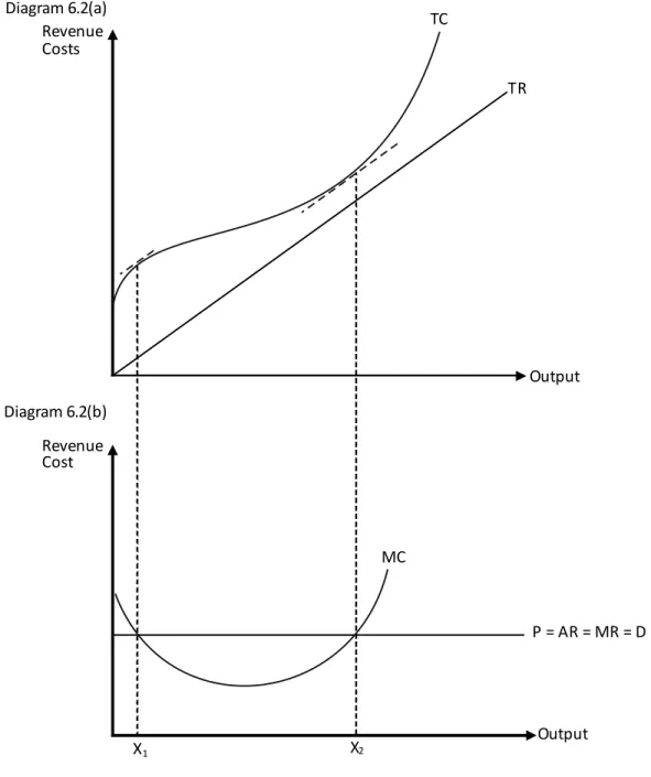
Thus, the intersection of increasing marginal cost and marginal revenue determines the profit-maximizing (or loss-minimizing) output. In Diagrams 6.1 (a & b), profit is maximized at X2 units of output, and the total revenue and total cost curves become parallel here. A firm that is making losses should consider closing down, but may continue to operate in the short term if its losses are less than fixed costs (this concept is explained later in the section).
Decisions to Continue or Shutdown Businesses
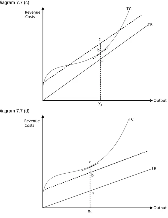
Firm C takes a loss (TR < TC), but this should continue in the short term as TR is greater than VC. This business should be continued in the short term because the losses are less than the fixed costs. In order to continue doing business in the long term, the sales revenue must be at least equal to the total costs.
Multiple Choice Questions (Section 6)
How much will an economist's calculation of the company's first year's costs exceed an accountant's calculation. 8 Which item would not appear in a company's financial accounts, but would be included in an economist's calculation of the company's costs. By how much would the economist's calculation of the company's total costs exceed an accountant's calculation of the company's total costs.
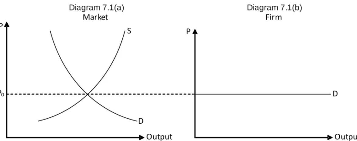
Perfect Competition
The following set of diagrams shows five possible short-run equilibria for a perfectly competitive firm. Thus, the short-run supply curve of a perfectly competitive firm is the increasing portion of MC over and above AVC. In Diagram 7.7 (d), the firm should shut down immediately because losses are higher than fixed costs.
Multiple Choice Questions (Section 7)
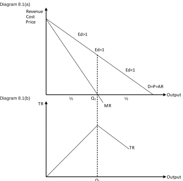
Therefore, a price cut increases total revenue (MR is positive) in the upper half and decreases it (MR is negative) in the lower half of the demand curve. The x-intercept of MR is exactly half of the demand curve (price or AR function). In the lower half of the demand curve (where demand is price inelastic), a profit-maximizing monopolist will always be tempted to raise the price that increases revenue and lowers total cost (since fewer units are sold at a higher price), thereby increasing profits.
Multiple Choice Questions (Section 8)
What can be deduced from this about the price elasticity of demand for the company's product. What will be the effect on the firm's revenue if it increases its price by 5. What will be the effect on the firm's revenue if it increases its price by 5%.
Negative Externalities
Marginal social cost is the cost that society incurs for producing an additional unit of the product. 9.1 the height of the demand curve shows the marginal social benefit (MSB) as well as the marginal private benefit (MPB). The firm maximizes its profit by producing Q1 where the private benefit of the last unit equals its private cost (MPB = MPC).
Positive Externalities
To minimize this, governments can impose heavier taxes on firms that use outdated technology and undesirable production methods. Governments can pass laws, restricting businesses from polluting the environment or creating other negative externalities. Governments can pass laws to ensure that production and consumption of products that carry positive externalities are increased.
Multiple Choice Questions (Section 9)
D The social costs of road transport are higher than the social costs of rail transport. 33 The diagram shows the private and social costs and benefits arising from the consumption and production of a good. Projects whose (discounted) social benefits exceed social costs are considered viable and can be implemented.
Multiple Choice Questions (Section 10)
7 Proper use of cost-benefit analysis should yield a result that minimizes social costs and maximizes social benefits. 8 What is an advantage of using cost-benefit analysis in decision-making, instead of using only private costs and private benefits? 11 In the cost-benefit analysis, the term net social benefit refers to a private benefit plus social benefit.
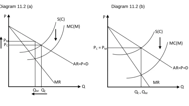
Section: 11 Comparison between Perfect Competition and Monopoly
A perfectly competitive company must be productively efficient in order to continue operating in the long run. Note that the assumption that the supply curve of a perfectly competitive market is similar to the monopoly's marginal cost (MC) curve ignores the possibility of economies of scale that a monopoly can exploit due to its size. The following set of diagrams shows how the transformation of a perfectly competitive industry into a monopoly affects market price and output.
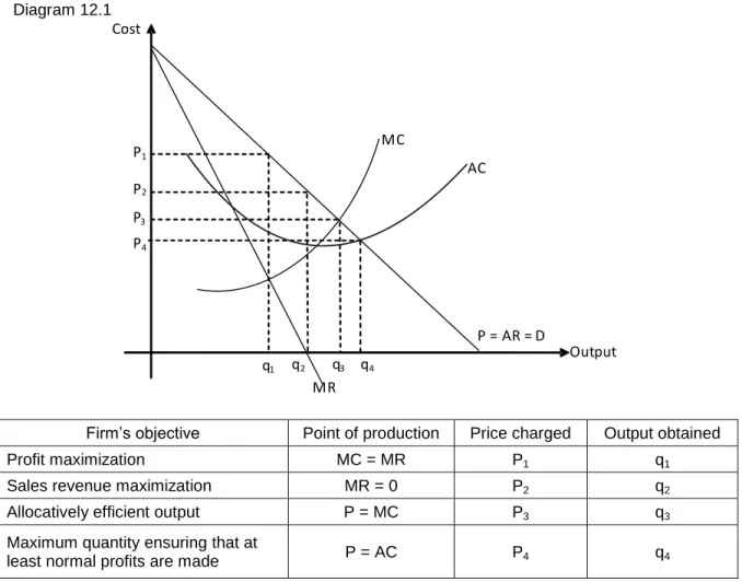
Efficiency: Productive and Allocative Efficiency
A firm is allocatively efficient when it charges a price equal to the marginal cost (MC) of the last unit produced. Consider a case where a firm is efficient but productively inefficient (for answers, consult the table in Section 14). Monopoly can be productively inefficient in both the short run and the long run (since it is possible to set a price higher than average cost).
Remedies to Monopoly Abuse
Like a unit tax, a unit subsidy applies to the number of units produced by the monopolist. A combination of a flat tax and a unit subsidy can be used to simultaneously achieve the goals of increasing production and reducing profits. A unit subsidy induces the monopolist to produce more, and a flat tax reduces profits.
Multiple Choice Questions (Section 11)
7 In the diagram, the introduction of a tax on goods causes the supply curve to shift from S1 to S2. 34 In the diagram, the introduction of a tax on goods causes the supply curve to shift from S1 to S2. 68 In the diagram, the introduction of a special tax causes the industry supply curve to shift from S1 to S2.
Multiple Choice Questions (Section 12)
A an increase in the price of the company's product B a decrease in the price of the company's shares C a decrease in the company's market share. A set a price for OX in the short and long term. B set a price for OY in the short and long term. What would the firm's increase in output be if it had to charge a price equal to its marginal cost?