Understanding Forward
Exchange Rates for Currency
In this chapter, we discuss forward contracts in perfect financial markets. Specif- ically, we assume that there are no transactions costs; there are no taxes, or at least they are non-discriminatory: there is but one overall income number, with all capital gains and interest earned being taxable and all capital losses and interest paid deductible; there is no default risk; and people act as price takers in free and open markets for currency and loans or deposits. Most of the implications of mar- ket imperfections will be discussed in later chapters; in this chapter we provide the fundamental insights that need to be mildly qualified later.
In Section 1, we describe the characteristics of a forward contract and how forward rates are quoted in the market. In Section 2, we show, with a simple diagram, the relationship between the money markets, spot markets, and forward markets.
Using the mechanisms that enforce the Law of One Price, Section 3 then presents the Covered Interest Parity Theorem. Two ostensibly unconnected issues are dealt with in Section 4: how do we determine the market value of an outstanding forward contract, and how does the forward price relate to the expected future spot price.
We wrap up in Section 5.
4.1 Introduction to Forward Contracts
Basics
Let us recall, from the first chapter, the definition of a forward contract. Like a spot transaction, a forward contract stipulates how many units of foreign currency are to be bought or sold and at what exchange rate. The difference with a spot deal, of course, is that delivery and payment for a forward contract take place in the future (for example, one month from now) rather than one or two working days from now,
as in a spot contract. The rate that is used for all contracts initiated at timet and maturing at some future moment T is called the time-t forward rate for delivery dateT. We denote it asFt,T .
Like spot markets, forward markets are not organized exchanges, but over-the- counter (OTC) markets, where banks act as market makers or look for counterparts via electronic auction systems or brokers. The most active forward markets are the markets for 30 and 90 days, and contracts for 180, 270, and 360 days are also quite common. Bankers nowadays quote rates up to ten years forward, and occasionally even beyond that, but the very long-term markets are quite thin. Recall, lastly, that any multiple of thirty days means that, relative to a spot contract, one extra calendar month has to be added to the spot delivery date, and that the delivery date must be a working day. Thus, if day [t+ 2 plus n months] is not a working day, we may move forward to the nearest working day, unless this would make us change months: then we’d move back.
Example 4.1
A 180-day contract signed on Thursday March 2, 2006 is normally settled on Septem- ber 6. Why? The initiation day being a Thursday, the “spot” settlement date is Monday, March 6. Add 6 months; September 6, being a working day (Wednesday), then is the settlement date.
Market Conventions for Quoting Forward Rates
Forward exchange rates can be quoted in two ways. The most natural and simple quote is to give the actual rate, sometimes called theoutright rate. This convention is used in, for instance, The Wall Street Journal, theFrankfurter Allgemeine, and the Canadian Globe and Mail. The Globe and Mail is one of the few newspapers also quoting long-term rates, as Table 4.1 shows.
In Table 4.1, thecad/usdforward rate exceeds the spot rate for all maturities.
Traders would say that the usd trades at a premium. Obviously, if the cad/usd rate is at a premium, the usd/cadforward rates must be below theusd/cadspot rate; that is, the cadmust trade at a discount.
The second way of expressing a forward rate is to quote the difference between the outright forward rate and the spot rate—that is, quote the premium or discount.
A forward rate quoted this way is called a swap rate.1 Antwerp’s De Tijd, or the London Financial Times, for example, used to follow this convention. Since both newspapers actually showed bid and ask quotes, we will postpone actual excerpts from these newspapers until the next chapter where spreads are taken into consid-
1Confusingly, the terms swap contract and swap rate can have other meanings, as we shall explain in Chapter 7.
Table 4.1: Spot and Forward Quotes, Mid-market rates in Toronto at noon (Outright) (Swap rates)
Premium or discount, in cents CAD per USD USD per CAD CAD per USD USD per CAD
U.S. Canada spot 1.3211 0.7569
1monthforward 1.3218 0.7565 +0.07 –0.05
2 months forward 1.3224 0.7562 +0.13 –0.07
3 months forward 1.3229 0.7559 +0.18 –0.10
6 months forward 1.3246 0.7549 +0.35 –0.20
12 months forward 1.3266 0.7538 +0.55 –0.31
3 years forward 1.3316 0.7510 +1.05 –0.59
5 years forward 1.3579 0.7364 +3.68 –0.05
7 years forward 1.3921 0.7183 +7.10 –3.86
10 years forward 1.4546 0.6875 +13.36 –6.94
Source Globe and Mail.
eration. The rightmost two columns in Table 4.1 shows how The Globe and Mail quotes would have looked in swap-rate form. In that table, the sign of the swap rate is indicated by a plus sign or a minus sign. The Financial Times used to denote the sign as pm (premium) or dis (discount).
The origin of the term swap rate is the swap contract. In the context of the forward market, a swap contract is a spot contract immediately combined with a forward contract in the opposite direction.
Example 4.2
To invest in the usstock market for a few months, a Portuguese investor buysusd 100,000 at eur/usd 1.10. In order to reduce the exchange risk, she immediately sells forward usd 100,000 for ninety days, at eur/usd 1.101. The combined spot and forward contract—in opposite directions—is a swap contract. The swap rate, eur/usd 0.1(cent), is the difference between the rate at which the investor buys and the rate at which she sells.
To emphasize the difference between a stand-alone forward contract and a swap contract, a stand-alone forward contract is sometimes called an outright contract.
Thus, the two quoting conventions described above have their roots in the two types of contracts. Today, the outright rate and the swap rate are simply ways of quoting, used whether or not you combine the forward trade with a reverse spot trade.2
One key result of this chapter is that there is a one-to-one link between the swap
2Sometimes the swap rate is called the cost of the swap, but to financial economists that is a very dubious concept: at the moment the contract is initiated, both the spot and the forward part are zero-NPVdeals, that is, their market value is zero. So the swap rate is not the cost of the swap in the same way a stock price measures the cost of a stock. It is more like an accounting concept of cost, in the style of the interest being the cost of a loan.
rate and the interest rates for the two currencies. To explain this relation, we first show how the spot market and the forward market are linked to each other by the money markets for each of the two currencies. But first we need to agree on a convention for denoting risk-free returns.
Our Convention for Expressing Risk-free Returns
We adopt the following terminology: the (effective) risk-free (rate of) return is the simple percentage difference between the initial, time-tvalue and the final, time-T value of a nominally risk-free asset over that holding period.
Example 4.3
Suppose that you deposit clp 100,000 for four years and that the deposit will be worth clp 121,000 at maturity. The four-year effective (rate of) return is:
rt,T = 121,000−100,000
100,000 = 0.21 = 21 percent. (4.1) You can also invest for nine months. Suppose that the value of this deposit after nine months is 104,200. Then the nine-month effective return is:
rt,T = 104,200−100,000
100,000 = 0.042 = 4.2 percent. (4.2)
Of course, at any moment in time, the rate of return you can get depends on the time to maturity, which equals T −t = 4 years in the first example. Thus, as in the above examples, we always equip the rate of return, r, with two subscripts:
rt,T. In addition, we need to distinguish between the domestic and the foreign rate of return. We do this by denoting the domestic and the foreign return byrt,T and rt,T∗ , respectively.
It is important to understand that the above returns, 21 percent for four years and 4.2 percent for nine months, are not expressed on an annual basis. This is a deviation from actual practice: bankers always quote rates that are expressed on an annual basis. We shall call such aper annum (p.a.) percentage an interest rate. If the time to maturity of the investment or loan is less than one year, your banker will typically quote you a simple p.a. interest rate. Given the simplep.a. interest rate, you can then compute the effective return as:
rt,T = [time to maturity, in years]×[simple p.a. interest rate for that maturity].
(4.3) Example 4.4
Suppose that thep.a. simple interest rate for a three-month investment is 10 percent.
The time to maturity,T −t, is 1/4 years. The effective return, then, is:
rt,T = (1/4)×0.10 = 0.025. (4.4)
The convention that we adopt in this text is to express all formulas in terms of effective returns, that is, simple percentage differences between end values and initial values. One alternative would be to express returns in terms of per annum simple interest rates—that is, we could have written, for instance, (T −t)Rt,T, (where capital R would be the simple interest on a p.a. basis) instead of rt,T. Unfortunately, then all formulas would look more complicated. Worse, there are many other ways of quoting an interest rate in p.a. terms, such as interest with annual, or monthly, or weekly, or even daily compounding; or banker’s discount; or continuously compounded interest. To keep from having to present each formula in many versions (depending on whether you start from a simple rate, or a compound rate, etc.), we assume that you have already done your homework and have computed the effective return from your p.a. interest rate. Appendix 4.6 shows how effective returns can be computed if thep.a. rate you start from is not a simple interest rate.
That appendix also shows how returns shouldnot be computed.
Thus, in this section, we will consider four related markets—the spot market, the forward market, and the home and foreign money markets. One crucial insight we want to convey is that any transaction in one of these markets can be replicated by a combination of transactions in the other three. Let us look at the details.
4.2 The Relation Between Exchange and Money Mar- kets
We have already seen how, using the spot market, one type of currency can be transformed into another at time t. For instance, you pay home currency to a bank and you receive foreign currency. Think of one wad of hc bank notes being exchanged for another wad offcnotes. Or even better, since spot deals are settled second working days: think of a spot transaction as an exchange of two cheques that will clear two working days from now. As of now, we denote the amounts by HC and F C. To make clear that we mean amounts, not names, they are written as math symbols (full-sized and slanting), not asfcand fc, our notation for names of currency. Another notational difference between currency names and amounts is that F C and HC always get a time subscript. To emphasize the fact that, in the above example, the amounts are delivered (almost) immediately, we add the t (=
current time) subscript: you pay an amountHCtin home currency and you receive an amountFCt of foreign currency.
By analogy to our exchange-of-cheques idea for a spot deal, then, we can picture a forward contract as an exchange of two promissory notes, with face values HCT and FCT, respectively:
Example 4.5
Suppose you sell forwardusd100,000 ateur/usd0.75 for December 31. (Note that the quote defines the euro as the hc.) Then
• you commit to deliver usd 100,000, which is similar to signing a promissory note (pn) with face value FCT=usd 100,000 on Dec 31, and handing it over to the bank;
• the bank promises to pay you eur 75,000, which is similar to giving you a signedpn with face valueHCT=eur75,000 for that date.
Intimately linked to the exchange markets are the money markets for the home and foreign country, that is, the markets for short-term deposits and loans. A home- currency deposit ofgbp1m “spot”3for one year at 4 percent means that you pay an amount ofgbp1m to the bank now, and the bank pays you an amount gbp1.04m at time T. This is similar to handing over the spot money amount of HCt=1m in return for apnwith face value HCT=1.04m. Likewise, if you borrowgbp 10m at 6 percent over one year, this is tantamount to you receiving a cheque with face value HCt=gbp 10m in return for a promissory note with face valueHCT=gbp10.6m.
Graphical Representation of Chains of Transactions: an Example
For the remainder of this section, we take the Chilean Peso (clp) as our home currency and the Norvegian Crown (nok) as the foreign one. Suppose the spot rate is St=clp/nok 100, the four-year forward rate Ft,T=clp/nok 110, the clp four-year risk-free rate of return isrt,T=21 percent effective, and thenokone equals rt,T∗ =10 percent. Very often we will discuss sequences of deals, or combinations of deals. Consider, for example, an Chilean investor who has clp 100,000 to invest.
He goes for a nok deposit “swapped into clp”, that is, a nok deposit combined with a spot purchase and a forward sale. Let us see what the final outcome is:
Example 4.6
The investor converts hisclp100,000 into an amountNOKt, deposits these for four years, and sells forward the proceeds NOKT in order to obtain a risk-free amount of clpfour years from now. The outcome is computed as follows:
1. Buy spot nok: the input given to the bank is clp 100,000, so the output of the spot deal, received from the bank, is 100,000×1/100 = 1,000 Crown.
2. Invest these nok at 10 percent: the input into the money market operation isNOKt = 1,000, so after four years you will receive from the bank an output equal to 1,000×1.10 = 1,100 Crowns.
3A spot deposit or loan starts the second working day. For one-day deposits, one can also define the starting date as today (“overnight”), or tomorrow (“tomorrow/next”), but this must be made explicit, then. In all our examples, the deals are spot—the default option in real life, too.
3. This futurenokoutcome is already being sold forward att; that is, right now you immediately cover or hedge the nokdeposit in the forward market so as to make its time-T value risk free rather than contingent on the time-T spot rate. The input for this transaction isNOKT = 1,100, and the output inclp at timeT will be 1,100×110 = 121,000.
There is nothing difficult about this, except perhaps that by the time you finish reading Step 3 you’ve already half forgotten the previous steps. We need a way to make clear at one glance what this deal is about, how it relates to other deals and what the alternatives are. One step in the right direction is to adopt a notation like
HCt= 100,000
buy spot:
×1/100
z}|{→ FCt= 1,000
deposit:
×1.10
z}|{→ FCT = 1,100
sell frwd:
×110
z}|{→ HCT = 121,000 So the arrows show how you go from a spotclp position into a spotnokone (the spot deal), and so on. We can further improve upon this by arranging the amounts in a diagram, where each kind of position has a fixed location. There are four kinds of money in play: foreign and domestic, each coming in a day-tand a day-T version.
Let’s show these on a diagram, with hc on the left and fc on the right, and with timeton top and timeT below. Figure 4.1 shows the result for the above example.
We can now generalize. Suppose the spot rate is stillclp/nok100, the four-year forward rate clp/nok 110, the clp risk-free is 21 percent effective, and the nok one 10 percent. The diagram in Figure 4.2 summarises all transactions open to the treasurer. It is to be read as follows:
Figure 4.1: Spot/Forward/Money Market Diagram: Example 4.6
HCT = 121,000 FCT = 1,100
HCt= 100,000 START HERE
FCt= 1,000
×1.10
×110
×1/100
-
?
Figure 4.2: Spot/Forward/Money Market Diagram: the general picture
HCT FCT
HCt FCt
×1.211 ×1.21
HC money market
×1.101 ×1.10
FC money market
×110
×1/110 forward market
×100
×1/100 spot market
-
-
?
6 6
?
• Anyt-subscripted symbolHCt (FCt) refers to anamount of spot money; and any T-subscripted symbol HCT (FCT) refers to a T-dated known amount of money, e.g. promised under apn,A/P,A/R or deposit, or forward contract.
• Any possible transaction (spot or forward sale or purchase; home or foreign money-market deal) is shown as an arrow. A transaction is characterized by two numbers: (a) your position before the transaction, an input amount you surrender to the bank, and (b) your position after the transaction, the output amount you receive from the bank. The arrow starts from the (a) part and ends in the (b) part. For example,
– a move HCt→FCt refers tobuying fc—spot (see “t”) – a move FCT →HCT refers toselling fc—forward (see “T”) – a move HCt→HCT refers toinvesting orlending hc
– a move FCT → FCt refers to borrowing against a fc income—e.g. dis- counting afc pn.
• Next to each arrow we write the factor by which its “input” amount has to be multiplied to compute the “output” amount. Again: “input” is what you give to the bank (at eithertorT), “output” is what you receive from it.
The General Spot/Forward/Money Market Diagram
To use the diagram, first identify the starting position. This is where you have money right now—like FCT (: a customer will pay youfc in future, or a deposit will expire). Then determine the desired end point, like HCT (: you want future hcinstead; that is, you want to eliminate the exchange risk). Third, determine by which route you want to go from START to END. Lastly, follow the chosen route, sequentially multiplying the starting amount by all the numbers you see along the path.
Example 4.7
In Example 4.6, the path is HCt → FCt → FCT → HCT, and the end outcome, starting from HCt= 100,000 is immediately computed as
HCT = 100,000× 1
100×1.10×110 = 121,000. (4.5)
The alert reader will already have noted that this is a synthetic hc deposit, constructed out of afcdeposit and a swap, and that (here) it has exactly the same return as the direct solution. Indeed, the alternative route, HCt → HCT, yields 100,000×1.21 = 121,000. (Inimperfect markets this equivalence of both paths will no longer be generally true, as we shall see in the next chapter.)
Example 4.8
Suppose that a customer of yours will pay nok 6.5m at time T, four years from now, but you need cash Pesos to pay your suppliers and workers. You decide to sell forward, and take out a clp loan with a time-T value that, including interest, exactly matches the proceeds of the forward sale. How much can you borrow on the basis of this invoice without taking any exchange risk?
The path chosen isFCT(=nok6,500,000)→HCT →HCt, and it yields 6.5m×110× 1
1.21 =clp590,909,090.91. (4.6)
The clever reader will again eagerly point out that there is an alternative: borrow nok against the future inflow (that is, borrow such that the loan cum interest is serviced by thenok inflow), and convert the proceeds of the loan intoclp. Again, in our assumedly perfect market, the outcome is identical: 6.5m/1.10 ×100 = clp590,909,090.91. Thus, the diagram allows us to quickly understand the purpose, and see the outcome of, a sequence of transactions. It also shows there are always two routes that lead from a given starting point to a given end point—a useful insight for shopping-around purposes. The advantage of using the diagram will be
even more marked when we add bid-ask spreads in all markets (next chapter) or when we study forward forwards or forward rate agreements and their relationship to forward contracts (Appendix 4.7),4 or when we explain forward forward swaps (Chapter 5).
4.3 The Law of One Price and Covered Interest Parity
The sequences of transactions that can be undertaken in the exchange and money markets, as summarized in Figure 4.2, can be classified into two types.
1. You could do a sequence of transactions that forms a roundtrip. In terms of Figure 4.2, a roundtrip means that you start in a particular box, and then make four transactions that bring you back to the starting point. For example, you may consider the sequenceHCT →HCt→FCt→FCT →HCT. In terms of the underlying transactions, this means that you borrow clp, convert the proceeds of the clploan into nok, and invest these nok; the proceeds of the investment are then immediately sold forward, back into clp. The question that interests you is whether the clp proceeds of the forward sale are more than enough to pay off the originalclp loan. If so, you have identified a way to make a sure profit without using any of your own capital. Thus, the idea behind a round-trip transaction isarbitrage, as defined in Chapter 3.
2. Alternatively, you could consider a sequence of transactions where you end up in a box that is not the same as the box from which you start. The two examples 4.7 and 4.8 describe such non-round-trip sequences. Trips like that have an economic rationale. In the first example, for instance, the investor wants to invest clp, and the question here is whether the swapped nok in- vestment (CLPt → NOKt → NOKT → CLPT) yields more than a direct clp investment (CLPt→ CLPT). Using the terminology of Chapter 3, this would be an example of shopping around for the best alternative.
In what follows, we want to establish the following two key results:
1. To rule out arbitrage in perfect markets, the following equality must hold:
Ft,T =St1 +rt,T
1 +rt,T∗ . (4.7)
[Inimperfect markets, this sharp equality will be watered down to a zone of admissible values, but the zone is quite narrow.]
4Forward Forwards and forward rate agreements (FRAs) are contracts that fix the interest rate for a deposit or loan that will be made (say) six months from now, for (say) three months. This can be viewed as a six-month forward deal on a (then) three-month interest rate. See the Appendix on forward interest rates.
Figure 4.3: Spot/Forward/Money Market Diagram: Arbitrage Computa- tions
121,000 1100
100.000 1000
×1.211 ×1.21
HC money market
×1.101 ×1.10
FC money market
×110
×1/110 forward market
×100
×1/100 spot market
-
-
?
6 6
?
2. If equation (4.7) holds, shopping-around computations are a waste of time since the two routes that lead from a given initial position A to a desired end position B produce exactly the same. Stated positively, shopping around can (and will) be useful only because of imperfections.
4.3.1 Arbitrage and Covered Interest Parity
In this section, we use an arbitrage argument to verify equation (4.7), a relationship called theCovered Interest Parity (CIP) Theorem. The theorem is evidently satisfied in our example:
110 =Ft,T =St1 +rt,T
1 +rt,T∗ = 1001.21
1.10 = 110. (4.8)
Arbitrage, we know, means full-circle roundtrips through the diagram. There are two ways to go around the entire diagram: clockwise, and counterclockwise. Follow the trips on Figure 4.3, where the symbols for amounts have been replaced by the specific numbers used in the numerical examples. We should not make any profit if the rate is 110, and we should make free money as soon as the rate does deviate.
Clockwise roundtrip The starting point of a roundtrip is evidently immaterial, but let’s commence with ahcloan: this makes it eminently clear that no own capital is being used. Also the starting amount is immaterial, so let’s pick an amount that produces conveniently round numbers all around: we write a pn with face value
CLPT = 121,000. We discount this,5 and convert the proceeds of this loan into Crowns, which are invested. At the same moment we already sell forward the future Crown balance. The final outcome is:
121,000× 1 1.21 × 1
100×1.10×110 = 121,000. (4.9) So we break exactly even: the forward sale nets us exactly what we need to pay back the loan.
DoItYourself problem 4.1
Show, similarly, that also the counterclockwise roundtrip exactly breaks even. For your convenience, start by writing apn with face valueNOKT = 1100. What is the path? What is the outcome?
What if Ft,T = too low, say 109? If one price is too low relative to another price (or set of other prices), we can make money by buying at this too-low rate.
The trip where we buy forward is the counterclockwise one. We start as before, except for the new price in the last step:
1100× 1
1.10 ×100×1.21× 1
109 = 1110.09>1100. (4.10) So the forward purchase nets us 1110.09 Pesos, 10.09 more than the 1100 we need to pay back loan.
DoItYourself problem 4.2 :
What if Ft,T is too high, say 111? Indicate the path and calculate the arbitrage profit.
DoItYourself problem 4.3
To generalize these numerical results, we now start withpn’s with face value 1, and replace all rates by their symbols. One no-arb condition is that the proceeds of the clockwise trip should not exceed the starting amount, unity. Explain how this leads to the following expression:
1 1 +rt,T
× 1 St
×(1 +rt,T∗ )×Ft,T ≤1. (4.11)
5Discounting apnor a T-bill or a trade bill not only means computing its PV; it often means borrowing against the claim. In practice, under such a loan the borrower would typically also cede the claim to the financier, as security. This lowers the lender’s risk and makes the loan cheaper.
This produces an inequality constraint, Ft,T ≤ St1+r1+rt,T∗
t,T. Write the no-arbitrage- profit condition for the counterclockwise trip and express it as another inequality constraint. Lastly, derive CIP.
4.3.2 Shopping Around (The Pointlessness of —)
The diagram in Figure 4.2 also tells us that any non-round-trip sequence of trans- actions can be routed two ways. For instance, you can go directly from CLPt to CLPT, or you can go viaNOKtandNOKT. In two earlier examples, 4.7 and 4.8, we already illustrated our claim that, in perfect markets whereCIPholds, both ways to implement a trip produce exactly the same outcome. It is simple to show that this holds for all of the ten other possible trips one could think of, in this diagram; but it would also be so tedious that we leave this as an exercise to any non-believer in the audience. It would also be a bit pointless, because in reality shopping around does matter. As we show in the next chapter, the route you choose for your trip may matter because of imperfections like bid-ask spreads, taxes (if asymmetric), information costs (if leading to inconsistent risk spreads asked by home and foreign banks), and legal subtleties associated with swaps.
4.3.3 Unfrequently Asked Questions on CIP
Before we move on to new challenges like the market value of a forward contract and the relation of the forward rate with expected future spot rates, a few crucial comments are in order. We first talk about causality, then about why pros always quote the swap rate rather than the outright, and lastly about taxes.
Covered Interest Parity and Causality
As we have seen, in perfect markets the forward rate is linked to the spot rate by pure arbitrage. Such an arbitrage argument, however, does not imply any causality.
CIP is merely an application of the Law of One Price, and the statement that two perfect substitutes should have the same price does not tell us where that “one price” comes from. Stated differently, showing Ft,T as the left-hand-side variable (as we did in Equation [4.7]), does not imply that the forward rate is a “dependent”
variable, determined by the spot rate and the two interest rates. Rather, what Covered Interest Parity says is that the four variables (the spot rate, the forward rate, and the two interest rates) are determined jointly, and that the equilibrium outcome should satisfy Equation [4.7]. The fact that the spot market represents less than 50 percent of the total turnover likewise suggests that the forward market is not just an appendage to the spot market. Thus, it is impossible to say, either in theory or in practice, which is the tail and which is the dog, here.
Figure 4.4: Appending Underlying Stories to the Variables inCIP
P. Sercu and R. Uppal The International Finance Workbook page 3.23
5.4 Causality in/around CIP? : one possible story
5. More on CIP
expected spot rate
risks of future spot rate expected
inflation, abroad business conditions (incl risk), abroad
S
rexpected inflation, home business conditions (incl risk), home
t t,T
r*t,T
Ft,T
AlthoughCIPitself does not say which term causes which, many economists and practitioners do have theories about one or more terms that appear in the Covered Interest Parity Theorem. One such theory is the Fisher equation, which says that interest rates reflect expected inflation and the real return that investors require.
Another theory suggests that the forward rate reflects the market’s expectation about the (unknown) future spot rate, ˜ST.6 We shall argue in Section 4.4 that the latter theory is true in a risk-adjusted sense. In short, while there is no causality in
CIP itself, one can append stories and theories to items in the formula. Then CIP
becomes an ingredient in a richer economic model with causality relations galore—
but S, F, r and r∗ would all be endogenous, determined by outside forces and circumstances. Figure 4.4 outlines a plausible causal story of how interest rates and the forward rate are set and, together, imply the spot rate.
CIP and the Swap Rate
When the forward rate exceeds the spot rate, the foreign currency is said to beat a premium. Otherwise, the currency isat a discount (Ft,T < St), orat par (Ft,T =St).
In this text, we often use the word premium irrespective of its sign; that is, we treat the discount as a negative premium. From [4.7], the sign of the premium uniquely
6We use a tilde (˜.) above a symbol to indicate that the variable is random or uncertain.
depends on the sign of rt,T −rt,T∗ :
[swap rate]t,T def= Ft,T −St,
= St
"
1 +rt,T 1 +r∗t,T −1
# ,
= St
"
1 +rt,T
1 +r∗t,T −1 +r∗t,T 1 +r∗t,T
# ,
= St
"
rt,T−rt,T∗ 1 +rt,T∗
#
; (4.12)
⇒ ∂·
∂St =
"
rt,T−r∗t,T 1 +rt,T∗
#
≈rt,T−r∗t,T. (4.13)
Thus, a higher domestic return means that the forward rate is at a premium, and vice versa. To a close approximation (with low foreign interest rates and/or short maturities), the percentage swap rate even simply is the effective return differential.
To easily remember this, think of the following. If there would be a pronounced premium, we would tend to believe that this signals an expected appreciation for the foreign currency.7 That is, the foreign currency is “strong”. But strong currencies are also associated with low interest rates: it’s the weak moneys that have to offer high rates to shore up their current value. In short, a positive forward premium goes together with a low interest rate because both are traditionally associated with a strong currency.
A second corollary from theCIPtheorem is that, whenever the spot rate changes, all forward rates must change in lockstep. In old, pre-computer days, this meant quite a burden to traders/market makers, who would have to manually recompute all their forward quotes. Fortunately, traders soon noticed that the swap rate is relatively insensitive to changes in the spot rate. That is, when you quote a spot rate and a swap rate, then you make only a small error if you do not change the swap rate every time S changes.
Example 4.9
Let the p.a. simple interest rates be 4 and 3 percent (hc and fc, respectively). If St changes from 100 to 100.5—a huge change—the theoretical one-month forward changes too, and so does the swap rate, but the latter effect is minute:
7Empirically, the strength of a currency is predicted by the swap rate only in the case of pro- nounced premia. When interest are quite similar and expectations rather diffuse, as is typically the case among OECD mainstream countries, the effects risk premia and transaction costs appear to swamp any expectation effect. See Chapter 10.
spot forward swap rate level0 100.0 100.0×1.0033331.002500 = 100.0831 0.0831 level1 100.5 100.5×1.0033331.002500 = 100.5835 0.0835
change 0.5 0.5004 0.0004
The rule of thumb of not updating the swap rate all the time used to work reason- ably well because, in olden days, interest rates were low8 and rather similar across currencies (the gold standard, remember?), and maturities short. This makes the fraction on the right hand side of [4.12] a very small number. In addition, interest rates used to vary far less often than spot exchange rates. Nowadays, of course, computers make it very easy to adjust all rates simultaneously without creating arbitrage opportunities, so we no longer need the trick with the swap rates. But while the motivation for using swap rates is gone, the habit has stuck.
DoItYourself problem 4.4
Use the numbers of Example 4.9 to numerically evaluate the partial derivative in Equation [4.13],
∂(Ft,T−St)
∂St =
"
rt,T−rt,T∗ 1 +rt,T∗
#
≈rt,T−rt,T∗ .
Check whether this is a small number, when interest rates are low (and rather similar across currencies) and maturities short. (If so, it means that the swap rate hardly changes when the spot rate moves.) Also check that the analytical result matches the calculations in the Example.
We now bring up an issue we have been utterly silent about thus far: taxes.
CIP: Capital Gains v Interest Income, and Taxes
When comparing the direct and synthetichcdeposits, in Example 4.7, we ignored taxes. This, we now show, is fine as long as the tax law does not discriminate between interest income and capital gains.
8During the Napoleonic Wars, for instance, theukissued perpetual (!) debt (the consolidated war debt, orconsol) with an interest rate of 3.25 percent. Toward the end of the nineteenth century, Belgium issued perpetual debt with a 2.75 percent coupon (to pay off a Dutch toll on ships plying for Antwerp). Rates crept up in the inflationary 70s to, in some countries, 20 percent short-term or 15 percent long-term around 1982. They then fell slowly to quite low levels, as a result of falling inflation, lower government deficits and, in the first years of the 21st century, high uncertainty and a recession—the “flight for safety” effect.
Table 4.2: HC and swapped FC investments with nondiscriminatory taxes Investclp 100 Invest nok1 and hedge
initial investment 100 1 ×100 = 100
final value 100×1.21 = 121 [1× 1.10]×110 = 121
income 21 21
interest 21 [1×0.10]×110 = 11
capgain 0 110 – 100 = 10
taxable 21 21
tax (33.33 %) 7 7
after-tax income 14 14
The first point you should be aware of is that, by going for a swappedfcdeposit instead of a hc one, the total return is in principle unaffected but the relative weight of the interest and capital-gain components is changed. Consider our Chilean investor who compares an investment innokto one in clp. Given the spot rate of 100, we consider investments of 100 clp or 1 nok. In Table 4.2 you see that the clpinvestment yields interest income only, while thenokdeposit earns interest (10 pence, exchanged at the forward rate 110) and a capital gain (you buy the principal at 100, and sell later at 110). But in both cases, total income is 21. (This, indeed, is the origin of the name CIP: the return, covered, is the same.)
DoItYourself problem 4.5
Verify that the expression below follows almost immediately from CIP, Equation [4.7]:
Ft,Trt,T∗ + (Ft,T −St) =Strt,T. (4.14) Then trace each symbol in the formula to the numbers we used in the numerical example. Identify the interest on the Peso and Crown deposits, and the capital gain or loss.
So we know that total pre-tax income is the same in both cases. If all income is equally taxable, the tax is the same too, and so must be the aftertax income. It also follows that if, because ofe.g. spreads, there is a small advantage to, say, the Peso investment, then taxes will reduce the gain but not eliminate it. That is, if Pesos would yield more before taxes, then they would also yield more after taxes.
In most countries, corporate taxes are neutral between interest income and capital gains, especially short-term capital gains. But there are exceptions. Theukused to treat capital gains onfc loans differently from capital losses and interest received.
Under personal taxation, taxation of capital gains is far from universal, and/or long- term capital gains often receive beneficial treatment. In cases like this, the ranking
of outcomes on the basis of after-tax returns could be very different from the ranking on pre-tax outcomes. Beware!
4.4 The Market Value of an Outstanding Forward Con- tract
In this and the next section, we discuss the market value of a forward contract at its inception, during its life, and at expiration. As is the case for any asset or portfolio, the market value of a forward contract is the price at which it can be bought or sold in a normally-functioning market. The focus, in this section, is on the value of a forward contract that was written in the past but that has not yet matured. For instance, one year ago (at timet0), we may have bought a five-year forward contract for nok at Ft0,T = clp/nok 115. This means that we now have an outstanding four-year contract, initiated at the rate ofclp/nok115. This outstanding contract differs from a newly signed four-year forward purchase because the latter would have been initiated at the now-prevailing four-year forward rate, clp/nok 110.
The question then is, how should we value the outstanding forward contract?
This value may be relevant for a number of reasons. At the theoretical level, the market value of a forward contract comes in quite handy in the theory of options, as we shall see later on. In day-to-day business, the value of an outstanding contract can be relevant in, for example, the following circumstances:
• If we want to negotiate early settlement of the contract, for instance to stop losses on a speculative position, or because the underlying position that was being hedged has disappeared.
• If there is default and the injured party wants to file a claim.
• If a firm wishes to “mark to market” the book value of its foreign-exchange positions in its financial reports.
4.4.1 A general formula
Let us agree that, unless otherwise specified, “a contract” refers to a forward pur- chase of one unit of foreign currency. (This is the standard convention in futures markets.) Today, at timet, we are considering a contract that was signed in the past, at timet0, for delivery of one unit of foreign currency to you atT, against payment of the initially agreed-upon forward rate,Ft0,T. Recall the convention that we have adopted for indicating time: the current date is always denoted byt, the initiation date byt0, the future (maturity) date by T, and we have, of course,t0 ≤t≤T.
The way to value an outstanding contract is to interpret it as a simple port- folio that contains a fc-denominated pn with face value 1 as an asset, and a hc- denominated pn with face value Ft0,T as a liability. Valuing ahc pn is easy: just
discount the face value at the risk-free rate. For the fc pn, we first compute its PV
infc (by discounting at r∗), and then translate thisfc value into hc via the spot price:
Example 4.10
Consider a contract that has 4 years to go, signed in the past at a historic forward price of 115. What is the market value ifSt= 100, rt,T = 21%, r∗t,T = 10%?
• The asset leg is like holding apn offc1, now worth PV* = 1/1.10 = 0.90909 nokand, therefore, 0.9090909×100 = 90.909 clp.
• The liability leg is like having written apnofhc115, now worthclp115/1.21
= 95.041.
• The net value now is, therefore,clp 90.909 – 95.041 = –4.132
The generalisation is as follows:
"Market value of forward purchase atFt0,T
#
=
PV* of as- set,fc1
z }| {
1
1 +rt,T∗ ×St
| {z }
translated value offcasset
− Ft0,T 1 +rt,T
| {z }
PV of hc liability
. (4.15)
There is a slightly different version that is occasionally more useful: the value is the discounted difference between the current and the historic forward rates. To find this version, multiply and divide the first term on the right of [4.15] by (1 +rt,T), and useCIP:
"Market value of forward purchase atFt0,T
#
= 1
1 +rt,T
1 +rt,T
1 +r∗t,TSt
| {z }
=Ft,T,(CIP)
− Ft0,T
1 +rt,T
= Ft,T−Ft0,T
1 +rt,T (4.16)
Example 4.11
Go back to Example 4.10. Knowing that the current forward rate is 110, we imme- diately find a value of (110 – 115)/1.21 = –4.132 clp for a contract with historic rate 115.
One way to interpret this variant is to note that, relative to a new contract, we’re overpaying by clp 5: last year we committed to paying 115, while we would have
gotten away with 110 if we had signed right now. This “loss”, however, is dated 4 years from now, so itsPV is discounted at the risk-free rate.
The sceptical reader may object that this “loss” is very fleeting: its value changes every second; how comes, then, that we can discount at the risk-free rate? One answer is that the value changes continuously because interest rates and (especially) the spot rate are in constant motion, But that does not invalidate the claim that we can always value each pn using the risk-free rates and the spot exchange rate prevailing at that moment. Relatedly, the future loss relative to market conditions attcan effectively be locked in at no cost, by selling forward for the same date:
Example 4.12
Consider a contract that has four years to go, signed in the past at a historic forward price of 115, for speculative purposes. Right now you see there is a loss, and you want to close out to avoid any further red ink. One way is to sell forward hc1 at the current forward rate, 110. On the common expiry date of old and new contract we then just net the loss of 115–110:
hcflows atT fc flows atT old contract: buy atFt0,T=115 –115 1 new contract: sell at Ft0,T=110 110 –1
net flow –5 0
But because this loss is realized within four years only, itsPVis found by discounting.
Discounting can be at the risk-free rate since, as we see, the locked-in loss is risk free.
We can now use the result in Equation [4.15] to determine the value of a forward contract in two special cases: at its inception and at maturity.
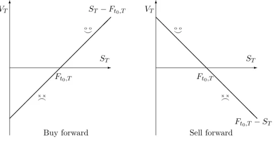
4.4.2 Corollary 1: The Value of a Forward Contract at Expiration At its expiration time, the market value of a purchase contract equals the difference between the spot rate that prevails at time T—the value of what you get—and the forward rate Ft0,T that you agreed to pay:
"Expiration value of a forward contract with rateFt0,T
#
=ST −Ft0,T. (4.17) Equation [4.17] can be derived formally from Equation [4.15], using the fact that the effective return on a deposit or loan with zero time to maturity is zero (that is, rT ,T = 0 =r∗T ,T. The result in [4.17] is quite obvious, as the following example shows:
Example 4.13
• You bought forward, at time t0, onenok atclp/nok 115. At expiry,T, the nok spot rate turns out to be clp/nok 123, so you pay 115 for something you can immediately re-sell at 123. The net value is, therefore, 123-115=8.
• Idem, except that ST turns out to be clp/nok 110. You have to pay 115 for something worth only 110. The net value is, therefore, 110-115=–5: you would be willing to pay 5 to get out of this contract.
The value of a unit forward sale contract is, of course, just the negative of the value of the forward purchase: forward deals are zero-sum games. The seller wins if the spot value turns out to be below the contracted forward price, and loses if the spot value turns out to be above. Figure 4.5 pictures the formulas, with smileys and frownies indicating the positive and negative parts.
Equation [4.17] can be used to formally show how hedging works. Suppose that you have to pay one unit of foreign currency at some future time T. The foreign currency debt is risky because the cash flow at time T, in home currency, will be equal to minus the future spot rate—and, at time t, this future spot rate is uncertain, a characteristic we stress by adding a tilde (∼) over the variable. By adding a forward purchase, the combined cash flow becomes risk free, as the bit of arcane math shows, below:
Cash flow from amortizing the debt at expiration: −S˜T Value of the forward purchase at expiration: S˜T −Ft0,T Combined cash flow: −Ft0,T.
(4.18) Putting this into words, we say that hedging the foreign-currency debt with a for- ward purchase transforms the risky debt into a risk-free debt, with a known outflow
Figure 4.5: The Value of a Forward Purchase or Sales Contract at Expiry
VT 6
- ST Ft0,T
ST −Ft0,T
^o o
_x x
Buy forward
VT 6
- ST Ft0,T
Ft0,T −ST
o o^
_x x
Sell forward
@
@
@
@
@
@
@
@
@
@
@
@
@@
−Ft0,T. We shall use this result repeatedly in Chapter 5 (on uses of forward con- tracts), in Chapter 9 when we discuss option pricing, and in Chapters 13 where we analyse exposure and risk management.
Make sure you realize that the hedged liability may make you worse off,ex post, than the unhedged one. Buying at a pre-set rateFt,T gives that great warm feeling, ex post, if the spot rate ST turns out to be quite high; but it hurts if the spot rate turns out to be quite cheap. The same conclusion was already implicit in [4.17]: the value of the contract at expiry can be either sign. This rises the question whether hedging is really so good as it is sometimes cracked up to be. We return to the economics of hedging in Chapter 12.
4.4.3 Corollary 2: The Value of a Forward Contract at Inception The value at expiry, above, probably was so obvious that it is, in a way, just a means of proving that the general valuation formula [4.15] makes sense. The same holds for the next special case: the value at inception, i.e. the time the contract is initiated or signed. At inception, the market value must be zero. We know this because (a) when we sign a forward contract, we have to pay nothing; and (b) hard- nosed bankers would never give away a positive-value contract for free, nor accept a negative-value contract at a zero price. To show the (initial) zero-value property formally, we use the general value formula [4.16] and consider the special case where t0 = t, implying that Ft0,T = Ft,T (That is, the contract we are valuing is new.) Obviously,
"Initial value of a forward contract with rateFt,T
#
= Ft,T −Ft,T 1 +rt,T
= 0. (4.19)
The value of a forward contract is zero at the moment it is signed because the contract can be replicated at zero cost. Notably, if a bank tried to charge you money for a contract at the equilibrium (Covered Interest Parity) forward rate, you would refuse, and create a synthetic forward contract through the spot and money markets:
Example 4.14
Let St = 100, r∗t,T = 0.10, rt,T = 0.21, Ft,T = 110; but a bank wants to charge you a commission of 3 for a forward purchase. You would shrug dismissively and immediately construct a synthetic forward contract at 110 at a zero cost:
• write apn adhc 110, discount it;
• convert the proceeds, 110/1.21 = 90.909090, intofc: you getfc0.90909.
• invest at 10 percent, to gethc 1 atT.
Thus, you can replicate a forward purchase contract under which your payment at T amounts to 110, just like in the genuine, direct forward contract, but it does not cost you anything now.
4.4.4 Corollary 3: The Forward Rate and the Risk-Adjusted Ex- pected Future Spot Rate
The zero-value property of forward contracts discussed above has another, and quite fundamental, interpretation. Suppose that the clp/nok four-year forward rate equals 110, implying that you can exchange one future nok for 110 future clp and vice versa without any up-front cash flow. This must mean that the market perceives these amounts as beingequivalent (that is, having the same value). If this were not so, there would have been an up-front compensation to make up for the difference in value.
Since any forward contract has a zero value, the present values of clp 1 four years and nok 110 four years must be equal anywhere; that is, the equivalence of these amounts holds for any investor or hedger anywhere. However, the equivalence property takes on a special meaning if we pick the clp (which is the currency in which our forward rate is expressed) as the home currency: in that particular num´eraire, the clp amount is risk-free, or certain. In terms of clp, we can write the equal-value property as:
PVt( ˜ST) = PVt(Ft,T), (4.20) where PVt(.) is the present-value operator. In a way, equation [4.20] is just the zero- value property: the present value of the uncertain future cash inflow ˜ST generated by the contract cancels out against the PV of the known future outflow, Ft,T. We can lose or gain, but these prospects balance out in present-value terms, from our time-t viewpoint. But the related, second interpretation stems from the fact that in home currency, the forward price on the right-hand side of Equation [4.20] is a risk-free, known number whereas the future spot rate on the left is uncertain. That is, at time t an amount of Ft,T Pesos payable at T is not just equivalent to one unit of foreign currency payable at T; this amount of future home currency is also acertain, risk-free amount. For this reason, we shall say that in home currency, the forward rate is the time-tcertainty equivalent of the future spot rate, ˜ST.
Example 4.15
In our earlier clp/nokexamples, the certainty equivalent of one Norvegian Crown four years out isclp110. You can offer the market a sureclp110 atT and get one Crown (with risky value ˜ST) in return; but equally well you can offer the market one Crown (with risky value ˜ST) and get a sure clp110 in return.
The notion of the certainty equivalent deserves some elaboration. Many in- troductory finance books discuss the concept of an investor’s subjective certainty equivalent of a risky income. This is defined as the single known amount of income that is equally attractive as the entire risky distribution.
Example 4.16
Suppose that you are indifferent between, on the one hand, a lottery ticket that pays
out with equal probabilities either usd100m or nothing, and on the other hand, a sure usd 35m. Then your personal certainty equivalent of the risky lottery is usd 35m. You are indifferent between 35m for sure and the risky cash flow from the lottery.
Another way of saying this is that, when valuing the lottery ticket, you have marked down its expected value,usd 50m, byusd15, because the lottery is risky.
Thus, we can conclude that your personal certainty equivalent, usd 35m, is the expected value of the lottery ticket corrected for risk.9
In the example, the risk-adjustment is quite subjective. A market certainty equivalent, by analogy, is the single known amount that the market considers to be as valuable as the entire risky distribution. And market certainty equivalents are, of course, what matter if we want to price assets, or if we want to make managerial decisions that maximize the market value of the firm. We have just argued that the (clp) market certainty equivalent of the future clp/nokspot rate must be the current clp/nok forward rate. Stated differently, the market’s time-t expectation of the time-T clp/nok spot rate, corrected for risk, is revealed in the clp/nok forward rate,Ft,T. Let’s express this formally as:
CEQt( ˜ST) =Ft,T, (4.21) where CEQt(.) is called the certainty equivalent operator.
A certainty equivalent operator is similar to an ordinary expectations operator, Et(.), except that it is a risk-adjusted expectation rather than an ordinary expected value. (There are good theories as to how the risk-adjusted and the “physical” den- sities are related, but they are beyond the scope of this text.) Like Et(.), CEQt(.) is also a conditional expectation, that is, the best possible forecast given the infor- mation available at time t. We use a t subscript to emphasize this link with the information available at timet.
To make the market’s risk-adjustment a bit less abstract, assume the CAPM holds. Then we could work out the left-hand side of [4.20] in the standard way:
thePVof a risky cashflow ˜ST equals its expectation, discounted at the risk-adjusted rate. The risk-adjusted discount rate, in turn, consists of the risk-free rate plus a risk premiumRPt,T(βS) which depends on market circumstances and the risk of the asset to be priced, βS. Working out the right-hand side of [4.20] is straightforward:
the PV of a risk-free flow F is F discounted at the risk-free rate r. Thus, we can
9When we say that investors are risk-avert, we mean they do not like symmetric risk for their entire wealth. The amounts in the example are so huge that they would represent almost the entire wealth of most readers; so in that case, risk aversion guarantees that the risk-adjustment is downward. But for small investments with, for instance, lots of right skewness, one observes upward adjustments: real-world lottery players, for instance, are willing to pay more than the expected value because, when stakes are small, right-skewness can give quite a kick.
flesh out [4.20] into
Et( ˜ST)
1 +rt,T +RPt,T(βS) = Ft,T 1 +rt,T
. (4.22)
After a minor rearrangement (line 1, below)we can then use the notationceqas in [4.21], to conclude that
Ft,T = Et( ˜ST) 1 +rt,T
1 +rt,T +RPt,T
⇒CEQt( ˜ST) = Et( ˜ST) 1 +rt,T
1 +rt,T +RPt,T (4.23)
≈ Et( ˜ST) 1 1 +RPt,T
. (4.24)
The last line is only an approximation of the true relation [4.23]. We merely add it to show why the fraction on the right-hand side of [4.23] is called the risk adjustment.
Example 4.17
Suppose your finance professor offers you a 1-percent share in the next-year royalties from his finance textbook, with an expected value, next year, of usd 3,450,000.
Given the high risk (^), the market would discount this at 10 percent—3 risk-freeo o plus a 7 risk premium. The ceqwould be
CEQ = 3,450,0001.03
1.10 = 3,450,000×0.936363636 = 3,090,000. (4.25) Thus, the market would be indifferent between this proposition and usd 3,090,000 for sure. You could unload either of these in the market at a common PV,
3,450,000
1.10 = 3,000,000 = 3,090,000
1.03 . (4.26)
The risk-adjusted expected value plays a crucial role in the theory of international finance. As we shall see in the remainder of this chapter and later in the book, the risk-adjusted expectation has many important implications for asset pricing as well as for corporate financial decisions.
4.4.5 Implications for Spot Values; the Role of Interest Rates In principle, we can see the spot value as the expected future value of the investment—
including interest earned—corrected for risk and then discounted at the appropriate risk-free rate. In this subsection we consider the role of interest rates and changes therein, hoping to clear up any confusion that might exist in your mind. Notably, we have noted that a forward discount, i.e. a relatively high foreign riskfree rate, signals a weak currency. Yet we see central banks increase interest rates when their
currency is under pressure, and the result often is an appreciation of the spot value.
How can increasing the interest rate, a sign of weakness, strengthen the currency?
The relation to watch is, familiarly,
St = CEQt( ˜ST)(1 +rt,T∗ )
1 +rt,T . (4.27)
We also need to be clear about what is changing, here, and what is held constant.
Let’s use an example to guide our thoughts.
Example 4.18
Assume that thecad(home currency) andgbprisk-free interest rates,rt,T andrt,T∗ , are both equal to 5 percentp.a. Then, from Equation [4.27], initially no change in S is expected, after risk adjustments: the spot rate is set equal to the certainty equivalent future value. Now assume that bad news about the British (foreign) economy suddenly leads to a downward revision of the expected next-year spot rate from, say, cad/gbp 2 to 1.9. From Equation [4.27], if interest rates remain unchanged, the current spot rate would immediately react by dropping from 2 to 1.9, too. Exchange rates, like any other financial price, anticipate the future.
Now if the Bank of England does not like this drop in the value of the gbp, it can prop up the current exchange rate by increasing the British interest rate. To do this, the uk interest rate will need to be increased from 5 percent to over 10.5 percent, so thatSt equals cad/gbp2 even though CEQt( ˜ST) equals 1.9:
1.9×1.10526
1.05 = 2. (4.28)
Thus, the higheruk interest rate does strengthen the currentgbpspot rate, all else being equal.
But this still means that the currency is weak, in the sense that thegbp is still expected to drop towards 1.9, after risk-adjustment, in the future. Actually, in this story the pound strengthens now so that it can become weak afterwards. So there is no contradiction, since “strengthening” has to do with the immediate spot rate (which perks up as soon as theukinterest rate is raised, holding constant theceq), while “weakening” refers to the expected movements in the future.
A second comment is that, in the example, the interest-rate hike merely post- pones the fall of the pound to a risk-adjusted 1.9. In this respect, however, this partial analysis may be incomplete, because a change in interest rates may also af- fect expectations. For instance, if the market believes that an increase in the British interest rate also heralds a stricter monetary policy, this would increase the expected future spot rate, and reinforce the effect of the higher foreign interest rate. Thus, the BoE would get away with a lower rise in the uk interest rate than in the first version of the story.
Of course, if expectations change in the opposite direction, the current spot rate may decrease even when the foreign interest rate is increased. For example, if the