Clα,mr Slope of lift curve of main rotor blade (rad−1) Clα,sb Slope of lift curve of stabilizer blade (rad−1) Clα,tr Slope of lift curve of tail rotor blade (rad−1) Clα,vf Lift curve slope of vertical rib ( rad−1) cmr Main rotor blade chord length (m). Kcol The ratio of the total pitch angle of the main rotor blades to the total servo pitch deflection (rad).
Introduction
Brief History of Rotorcraft
Then attention is paid to the development of larger scale, that is, miniature UAVs as well as their practical applications. The current popularity of miniature rotorcraft UAVs is largely contributed by the many research groups and companies that are actively conducting research in this area.
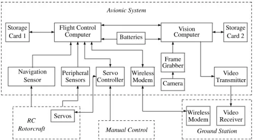
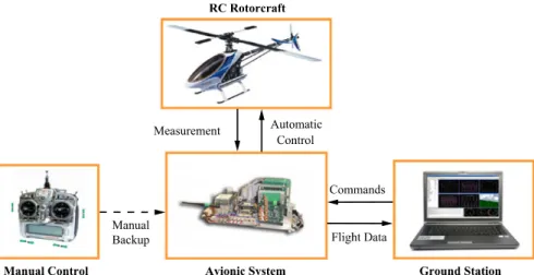
Essential Hardware Components
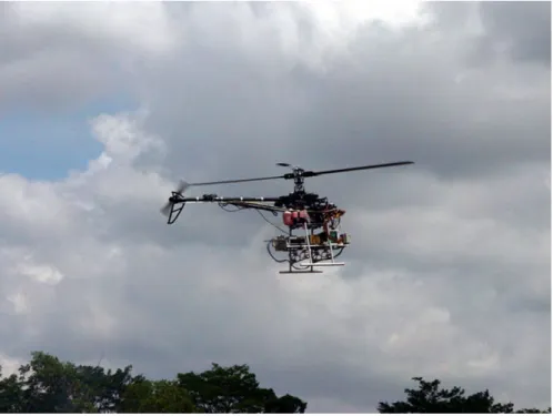
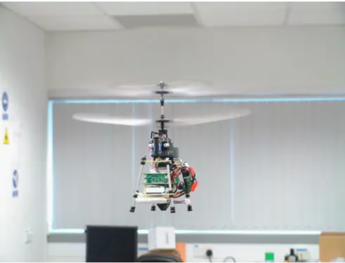
- RC Rotorcraft
- Avionic System
- Manual Backup
- Ground Control Station
The pin-socket connection on the PC/104(-plus) SBCs also provides greater compatibility for integrating additional modules, such as serial expansion cards, analog-to-digital (A/D) conversion cards, power regulator cards, and frame grabber boards (for image - and video conversion) into the system without reconfiguration. Most commercial magnetometers are MEMS-based and with sufficient resolution (milligauss level) and sampling rate (up to 10 Hz).
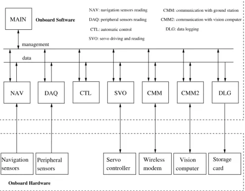
Software Design and Integration
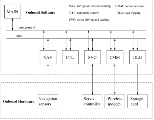
Avionic Real-Time Software System
The CMM is for communication between the avionics system and the ground station via wireless links. DLG is for data logging, which is usually created as a background task to save data during flight.
Ground Control Station Software Structure
Flight Dynamics Modeling
First-Principles Approach
The first-principles modeling approach is well developed for obtaining dynamic models for full-scale manned and unmanned rotorcraft. Some initial success, in which the first-principles modeling technique is applied to small-scale UAV helicopters, has been documented in the literature.
System and Parameter Identification
Flight Control Systems
In [18], the function of the inner-loop control law, designed using the H∞control approach, is to guarantee the asymptotic stability of the aircraft motion and to have good disturbance rejection with respect to wind gusts. The role of the outer loop is to produce flight commands or references to the inner loop control layer, and finally the task of the flight scheduling part is to generate the flight references for pre-scheduled flight missions.
Application Examples
Two representative examples of rotorcraft UAV application for combat arms support are the Autocopter Gunship [5] equipped with up to 2 AA-12 guns for air firing and the Schiebel S-100 equipped with light multi-role missiles ( LMM). Agriculture and Forestry A successful application of rotorcraft UAVs in the civil field is the spraying of pesticides in agriculture and forestry.

Preview of Each Chapter
Introduction
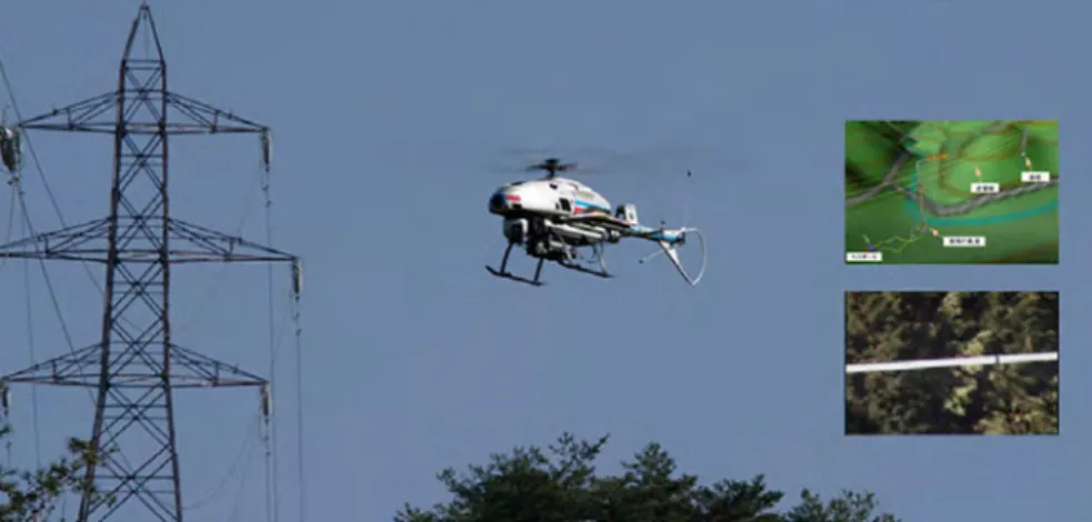
It is equipped in most miniature UAV engines to significantly increase safety in the air. Rotorcraft UAVs can also be of great help to civil defense and law enforcement (see, e.g., the case reported in [126]).
Coordinate Systems
- Geodetic Coordinate System
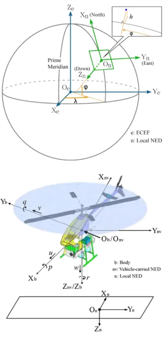
- Earth-Centered Earth-Fixed Coordinate System
- Local North-East-Down Coordinate System
- Vehicle-Carried North-East-Down Coordinate System
- Body Coordinate System
Coordinate vectors expressed in terms of the geodesic frame are denoted by a subscript g, i.e. the position vector in the geodetic coordinate system is denoted by . The origin (denoted Ob) is at the center of gravity (CG) of the flying vehicle.
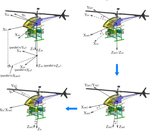
Coordinate Transformations
Fundamental Knowledge
YAW ANGLE, denoted by ψ, is the angle from the vehicle-borne NED X-axis to the projected vector of the body X-axis on the X-Y plane of the vehicle-borne NED frame. After this rotation (indicated by Rint1/nv), the vehicle-borne NED frame transitions to a one-time rotated intermediate frame.
Coordinate Transformations
The kinematic relationships between the NED carried by the vehicle and the body frames are important for flight dynamics modeling and automatic flight control. For rotational kinematics, we focus on the angular velocity vector ωbb/nv that describes the rotation of the NED frame carried by the vehicle with respect to the body frame projected onto the body frame.
Introduction
Virtual Design Environment Selection
Powerful 3D and 2D design: For any selected component, its virtual 3D counterpart can be precisely modeled in terms of shape, size and color. Precise physical description: Each virtual component can be parameterized with the necessary physical parameters such as size, dimension and weight.
Hardware Components Selection
- RC Helicopter
- Flight Control Computer
- Navigation Sensors
- Peripheral Sensors
- Fail-Safe Servo Controller
- Wireless Modem
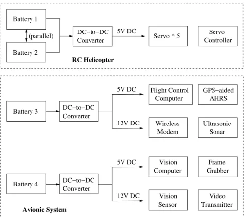
- Batteries
- Vision Computer
- Vision Sensor
- Frame Grabber
- Servo Mechanism
- Video Transmitter and Receiver
- Manual Control
- Ground Control Station
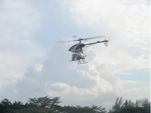
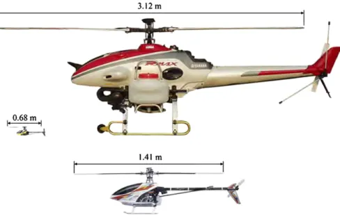
The principle of operation of the Raptor 90 SE (see Figure 3.4) is standard and widely accepted in the hobby community. The RPM sensor is used to provide the main rotor RPM in real time to the flight control computer.
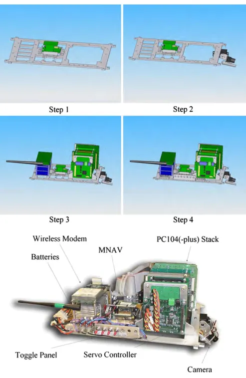
Avionic System Design and Integration
- Layout Design
- Anti-vibration Design
- Power Supply Design
- Shielding Design
We need to determine the correct positions of (i) the two PC/104(-plus) computers, (ii) the frame grabber, (iii) the servo controller board, (iv) the wireless modem, and (v) the batteries. We have carefully selected their mounting positions to achieve precise CG tuning of the aircraft system.
Performance Evaluation
Introduction
The Z axis (denoted Ze) is along the Earth's axis of rotation and points to the North Pole. The origin (denoted by Onv) is located at the center of gravity (CG) of the flying vehicle.
Onboard Software System
- Framework Design
- Task Management
- Implementation of Automatic Control
- Emergency Handling
- Vision Processing Software Module
Its time consumption depends entirely on the complexity of the algorithms used for the flight control system. Finally, we provide the time allocation for the threads of the vision software system tasks in Table 4.3.
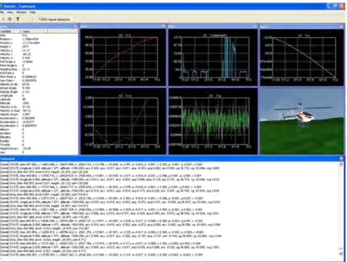
Ground Control Station Software
Framework of Ground Station Software Module
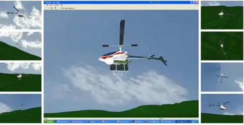
The development of the 3D rendering in our ground station (see e.g. [42]) includes (i) the creation of the 3D models of the helicopter and ground environment, (ii) the OpenGL (open graphics library) programs for kinematic transformations of these models, and finally (iii) the integration of the 3D display into the general ground station software system. It is linked to the globally shared data (i.e. the kernel layer), which stores the flight data of the UAV helicopter.
Software Evaluation
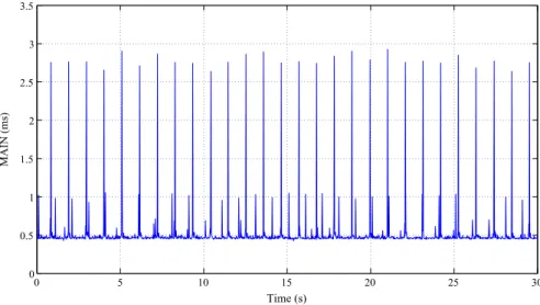
The times consumed by all task threads are summed in Figure 4.14 as the main thread's CPU time consumption. From the results shown in Figure 4.14, we can see that the lowest level of computer usage is for flight control.
Introduction
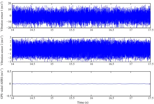
The goal of this chapter is to introduce an integration of a low-cost inertial attitude and position reference system for a mini-UAV helicopter by applying the well-known EKF technique. The overall procedure is summarized and depicted in Fig.5.1, which consists of two independent parts, one for AHRS and one for INS.
Extended Kalman Filtering
Prediction stage: The prediction stage uses the previous time step to produce an estimate of the state at the current time step [203]. If the initial estimate of the state is wrong, or if the given dynamic model is imprecise, the filter can quickly diverge due to its linearization.
Dynamics Models of the GPS-Aided AHRS
AHRS Dynamics Model
In particular, it is determined for the 3–2–1 Euler rotation series, where the items involved are given by . For the accelerometer, the output measurement vector corresponding to the correct measured acceleration i.e. amea is given by.
INS Dynamics Model
It should be noted that the above equation is only valid for small-scale aircraft performing normal maneuvers with a very small acceleration change (compared to the gravitational acceleration projections).
Design of Extended Kalman Filters
EKF for AHRS with Accelerometer Measurement
Based on the AHRS dynamics model with the accelerometer measurement as given by (5.23) and (5.24), we present below the detailed EKF parameters for the accelerometer-based AHRS signal enhancement. The numerical values assumed for the EKF of the accelerometer-based AHRS are given as respectively.
EKF for AHRS with Magnetometer Measurement
The Euler angles used in the above two equations are those updated in the previous time step, that is, timek−1. Signal Update: The signal update step is identical to its counterpart in the EKF associated with the accelerometer based AHRS.
EKF for INS
92 5 Measurement Signal Enhancement whereHx,nandHy,nres the horizontal magnetic field measurement in the local DOWN frame, and Hx,off andHy,off are the magnetic field measurement offsets projected onto the local DOWN frame, which are mainly caused by some minor EMI of the unmanned system and can be determined by calibrating hard and soft iron.
Performance Evaluation
Introduction
More specifically, the flight control computer shares the unmanned helicopter's underflight conditions with the vision computer. This layer communicates with the software module of the avionics system (ie the CMM task thread) through the wireless communication channel.
Model Structure
- Kinematics
- Rigid-Body Dynamics
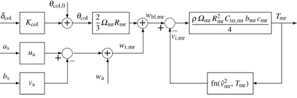
- Main Rotor Flapping Dynamics
- Yaw Rate Feedback Controller
This is in line with the main rotor dynamics focus we intend to study. The tail rotor creates thrust that opposes the fuselage torque resulting from the rotation of the main rotor.
Parameter Determination
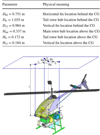
- Direct Measurement
- Ground Tests
- Estimation Based on Wind-Tunnel Data
- Flight Test
- Fine Tuning
We note that the lift curve slope of the main rotor blade, tail rotor blade and stabilizer bar can be further tuned in the last part of the proposed parameterization procedure. Among them, the first five are related to the mechanical model of the Bell-Hiller mixer, and the obtained parameters have sufficient reliability.
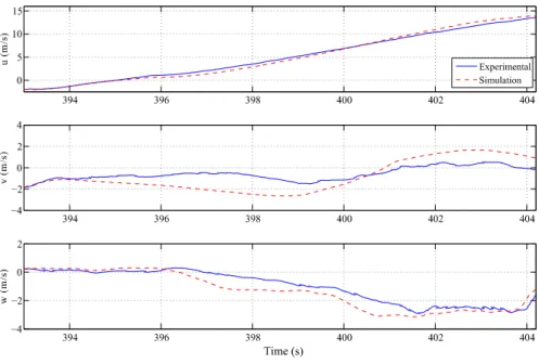
Model Validation
Based on the same inputs, we compare the experimental and simulation responses in terms of body frame velocities, Euler angles, and angular velocities. These problems can be overcome by a properly designed automatic flight control system, which will be addressed in later chapters.
Flight Envelope Determination
Furthermore, it assumes that the power requirement in a wide envelope is approximately the same as in hovering [91]. In fact, we conducted a series of manual flight tests and found that the practical speed limit for the SheLion is about 15 to 17 m/s.
Introduction
In this chapter, we present the design of the inner-loop control law using the H∞ control technique. As such, the H∞control method, a technique developed to attenuate external disturbances while maintaining closed-loop stability, is a natural choice for the inner control loop to realize both internal stabilization and disturbance rejection.
H ∞ Control Technique
Note that, for the state feedback case, the H∞γ-suboptimal control law is given by u=FxwithF which is given as in (7.15). Below is a step-by-step algorithm that constructs the reduced-order output feedback controller for general H∞ optimization.
Inner-Loop Control System Design
Model Linearization
Problem Formulation
Selection of Design Specifications
H ∞ Control Law
Performance Evaluation
Introduction
For example, main rotor flapping, due to the existence of the stabilizer bar, must be included in the modeling process.
Robust and Perfect Tracking Control
The full-order measurement output feedback controller that solves the RPT problem for the given system is given by . STEP R.4: The reduced order gauge feedback control law that solves the RPT control problem for the given system is then given by.
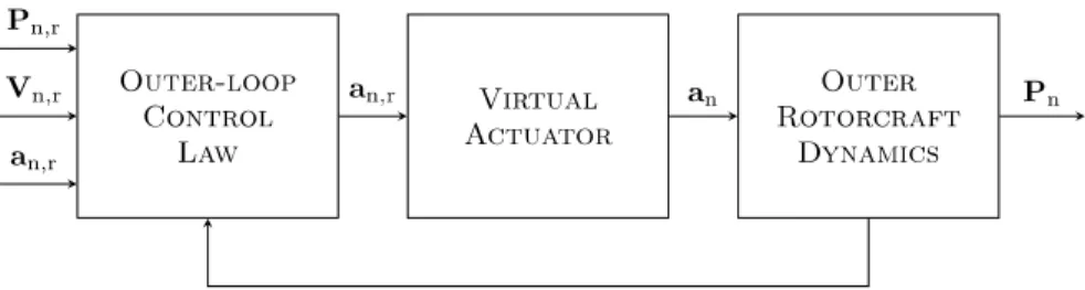
Outer-Loop Control System Design
Since all three channels share the same dynamic structure, we proceed in what follows to focus on designing the outer loop controller for the X-axis only using the RPT control technique introduced in the previous section. More specifically, the closed-loop eigenvalues of the X-axis dynamic system under state feedback control are given by .
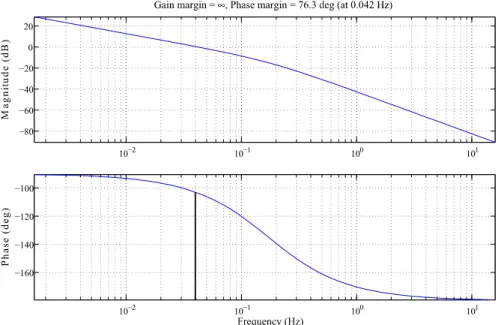
Performance Evaluation
However, due to the limitations of the physical system and the limitations of the inner loop dynamics, the response of the outer loop system must be slower than the bandwidth of the virtual actuator, i.e., 1 rad/s. For testing gust disturbance damping and tracking performance of the flight control system, we include the inner-loop controller of Chap.
Introduction
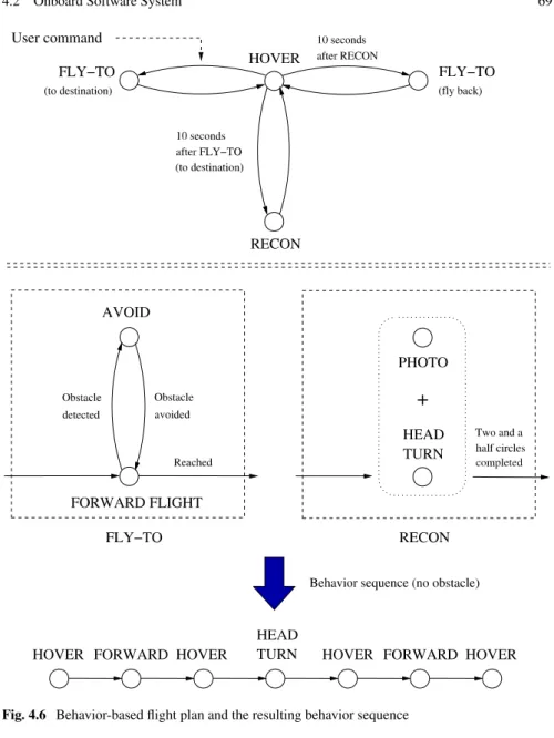
Flight Scheduling
Depart/Abort (Forward Flight)
Hover
Depart/Abort (Backward Flight)
Hovering Turn
Vertical Maneuver
Lateral Reposition
Turn-to-Target
Slalom
Pirouette
MTE Concatenation
Hardware-in-the-Loop Simulation Setup
Simulation and Flight Test Results
Introduction
Leader-Follower Formation
Coordinate Systems in Formation Flight
Kinematics Model
Collision Avoidance
Flight Test Results
Introduction
Coordinate Frames Used in Vision Systems
Camera Calibration
Camera Model
Intrinsic Parameter Estimation
Distortion Compensation
Simplified Camera Model
Vision-Based Ground Target Following
Target Detection
Image Tracking
Target Following Control
Experimental Results