Σpcd Covariance matrix of multivariate measurement uncertainty in PC space ΣD Covariance matrix of extended measurement distribution. Σz Covariance matrix of the extended distribution of model outputs Σzz Covariance matrix of the extended distribution z−z′.
Overview
The model is used to predict metal temperatures of the high-pressure turbine disc of a gas turbine engine during operation. When implementing VVUQ for practical modeling and simulation, consideration must be given to how the various sources of uncertainty will be aggregated so that meaningful error bounds can be assigned to model predictions—the intended use of the model.
Definitions for the VVUQ process
This is "the process of assessing software correctness and numerical accuracy of the solution to a given mathematical model" [2]. This is "the process of determining the degree to which a model is an accurate representation of the real world from the perspective of the intended uses of the model." [1, 16].
Research objectives and organization of the dissertation
Several studies have attempted to combine the contributions of different sources of error and uncertainty. Finally, a summary of the contributions of this thesis and recommendations for future work are discussed in Chapter 8.
An engineering physics model for application of the research methodologies
Basic model requirements
Thus, the steps in (ii) ensure the quality and accuracy of the model before the final prediction is made. This VVUQ framework is demonstrated to quantify uncertainty in the prediction of the primary QoI.
Conceptual model
System description and operation
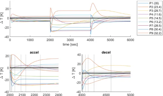
Therefore, the purpose of the model definition step is to ensure that the right physics is modeled, but to balance complexity with sufficiency to meet the requirements for an acceptable level of uncertainty. att = 2000 and t = 6000 seconds for idle, t = 4000 seconds for MTO), with rapid acceleration/deceleration maneuvers between conditions (Figure 2.3, bottom). This provides both steady-state and transient temperature characteristics for evaluating the model (Figure 2.3, top).
Phenomena identification and ranking table (PIRT)
Mathematical model
Uncertainty identification
Similar parameters can be applied to other aspects of the model boundary conditions, such as heat generation by air friction. Model parameters are an epistemic source of uncertainty since obtaining additional measurements (or measurements with reduced uncertainty) for model calibration would reduce the posterior uncertainty.
Computational model
Multivariate model output
However, due to the autocorrelation present in the time series output at each individual location, the dimension of the time series output can be reduced by extracting meaningful 'features' of the time-dependent response (reducing Rnts → Rnc). The time points include the two stabilized temperature time points (t= 2000 and t= 4000 seconds for idle and MTO, respectively) and are selected as above to characterize the steady-state response.
Test measurements for model calibration and validation
Therefore, in this research it is assumed that a 'known' (prescribed) measurement uncertainty is available, based on previous information or experience, in the form of a standard deviation σd. In this case, calibration can be performed using measurements from the first maneuver and validation using measurements from the second.
Conclusion
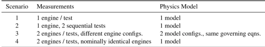
In the second scenario, the same engine is run through two different test cycles, for example the square cycle discussed above and another modified set of engine maneuvers. In the third and fourth scenarios, one test is used for calibration and the second test for validation.
Introduction
Richardson extrapolation
If the observed accuracy order is similar to the formal accuracy order, Fs = 1.25 is suggested, otherwise Fs = 3. It is also recommended to limit the range of the observed accuracy order when calculating this limit to 0.5≤ˆa≤ a ∗the while∗is the formal order of accuracy [2].
Challenges with Richardson extrapolation
Thomas et al [53] propose the use of "windowing" and "downsizing" which takes a region of the mesh and refines it semi-locally to allow uniform refinement so that asymptotic behavior can be achieved. The use of GP alleviates the practical challenges in RE for this application in two ways.
Methodology
Setting mesh levels
The internal code's adaptive mesh and time stepping routines are controlled by user-set error limits. However, the adaptive time step cannot be disabled, so the uniform refinement only applies to the spatial aspect and Et must also be specified, as described next.
GP based discretization error estimation (GPDE)
Demonstration of GPDE
- GPDE for uniform refinement compared to Richardson extrapolation
- GPDE for adaptive refinement
- Comparison of GPDE for uniform and adaptive refinement
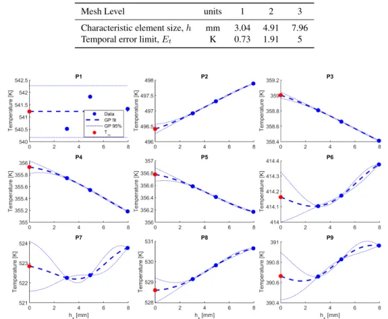
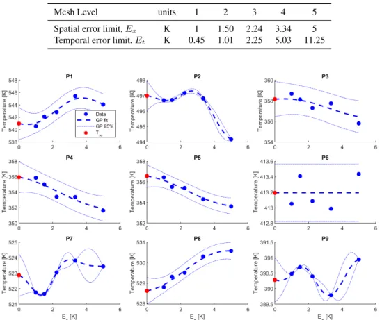
In cases where the GPs in Figure 3.3 are less well defined in the region of extrapolymyth→ 0 (eg, P1, P6, P7, P9), it is observed that the estimate of fˆ (red dot) shifts towards the average of the three network, the values of the level fkand its standard deviation increases towards the standard deviation of the three fk values. This also results in larger GPDE than the uniform case at some locations, as Figure 3.6 highlights.
Discretization errors and uncertainty aggregation
Conclusion
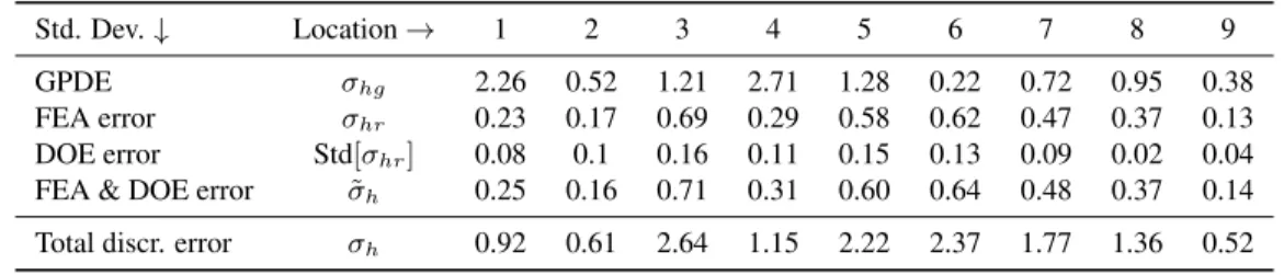
The methodology for quantifying the uncertainty in the discretization error estimate due to dependence on inputs/parameters (which are uncertain) relied on the recovery-based errors available in the FE solution DOE results.
Introduction
Since the results are uncorrelated, any of the methods based on scalar output can be used. iii). After formulating the surrogate PC-AS model, we demonstrate the Bayesian calibration of a thermal FE model of the gas turbine disk, followed by forward propagation of parameter uncertainties using standard Monte Carlo simulation.
Model definition
Heat transfer model outputs
In this chapter, the 6-node triangular element mesh contains 10,071 nodes (710 only for the turbine disk, the darkest gray domain in Figure 4.2). For the purpose of this study, these errors were considered acceptable and were not carried over to the calibration step.
Synthetic test measurements
In this case, the model execution time was fast (13 seconds per run of 16 models running in parallel, one model run per compute core). The FE code used in this analysis has an adaptive mesh and the ability to finer the time step to reach the selected error threshold.
Efficient surrogate modeling
- Output transformation with principal component analysis (PCA)
- Input transformation with active subspace (AS)
- The resulting PC-AS surrogate model
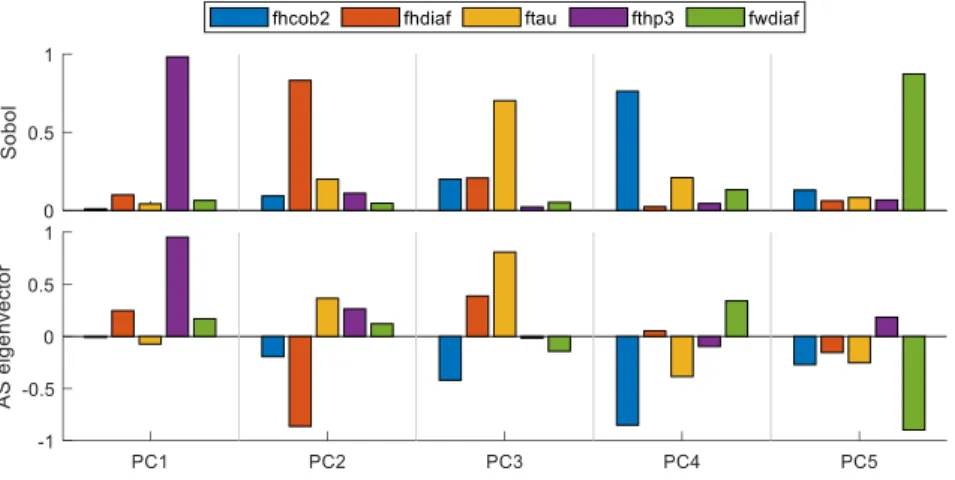
- Sensitivity analysis of PCs vs eigenvector
Since the LHS is used, ρ(θ) is interpreted as a uniform distribution of random variables θ, as in previous work which means, Cis the expected value (mean) of the outer product of the gradient. The shadow plots are outputsykpcplots of computational space as a function of the active subspace parameters wkTθ (blue dots), which are fit to surrogate quadratic polynomial regression models (red curves).
Application of the PC-AS surrogate in Bayesian calibration
- Bayes’ rule and setting up the calibration problem
- Markov chain Monte Carlo sampling
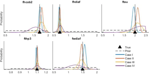
- Bayesian calibration results
- Forward propagation of the parameter posteriors
- Summary of the analysis process
First, the physical model is replaced by the PC-AS surrogate ≈ gs(x,θ) + ϵs, creating a Gaussian approximation for the surrogate model errorsϵs∼ N(0, σs) from the residuals of the fit in Figure 4.5. Several methods are available for the solution of Bayes' rule depending on the complexity of the posterior distribution.
Conclusion
Measurement noise (case II) and increased variance (case III) are clearly transferred to the results and show the same trends. The accuracy of the surrogate PC-AS model was high in the studied case (R2 = 0.95 for N >20 samples).
Introduction
However, in the modular approach, the error between the previous prediction and measurements is used as a starting point for the calibration of the discrepancy function. To the best of the authors' knowledge, there has been no previous research on model discrepancy functions in the PC space.
Background
Bayesian calibration with additive discrepancy
Then the methodology is applied to a gas turbine engine heat transfer model calibration problem in Section 5.4 and the chapter concludes in Section 5.5.
Assessing non-identifiability
Thus, V−1, which is diagonal due to the assumption of independent priors, adds a regularizing 'ridge' to the diagonal eXTΣ−1d X =σ12. Although this is also true for Bayesian inference, in the implementation of Section 5.4, we assume weakly informative (uniform) priors and therefore only use (XTX)-1 as the basis of the number of feasible parametersψ={θ,ϕ }that can be calibrated.
Methodology
- Bayesian calibration problem in PC space
- Selecting discrepancy functions in PC space
- Non-identifiability assessment in PC space
- Functional dependence in PC space
- Selected discrepancy functions
- Evaluating the selected discrepancy functions
- An illustrative model
- No discrepancy function (original space)
- Non-identifiable discrepancy function (original space)
- Identifiable discrepancy function (original space)
- Discrepancy function in PC space (non-identifiable)
- Use of the calibrated discrepancy
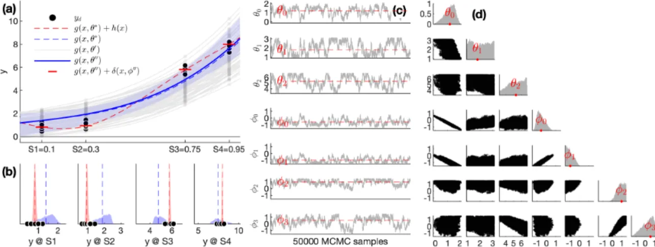
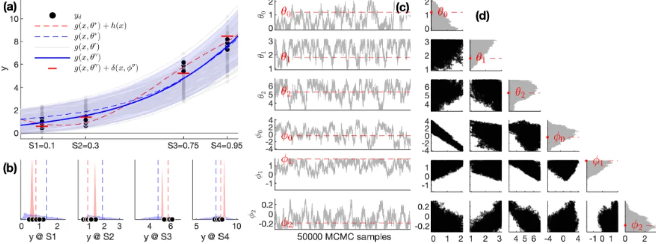
With respect to a true unknown solution (i.e., the real world), these criteria are not applicable, but can (i) test candidate models for parameter non-identifiability, (ii) check the posterior variance of the model uncorrected, (iii) compare predictions using posteriors and the corrected model on a 'keep out' validation dataset if available. Another observation in Figure 5.2 is that the corrected posterior solution matches the true solution very well, i.e., the red prediction histograms are centered on the red dashed true solution line in panel (b).
Application to the heat transfer model
- Synthetic measurements and model form error
- Selecting discrepancy functions
- Evaluating the discrepancy functions
- Use of the calibrated discrepancy for physics model diagnosis
Thus, the corrected output does not provide primary feedback on the calibration performance of the mismatch function. In contrast, Case 21 includes the MFE like most of the other cases, but has no mismatch function.
Conclusion
Therefore, it was proposed to instead use model misfit for diagnostic purposes in this application: perform a model calibration with and without a model misfit function included, then review the shifts in posterior and hindcasts for required boundary conditions that contribute to the source of the lack of physics in the model. Finally, Subramanian and Mahadevan demonstrate an alternative to the model output mismatch approach with intrusive [133] and non-intrusive [103] methods that estimate the model form error in the governing equations.
Introduction
There is limited guidance in the standards on how the validation assessment should be performed and used in subsequent analysis. The extended metric is demonstrated on a 2D numerical example (Section 6.3.4) and the gas turbine engine heat transfer model (Chapter 2) with multiple outputs (Section 6.4).
Background
Features of interest for the selection of validation metrics
The engineering literature points out the desirable properties that validation metrics should have and ways to classify types of validation metrics. For example, Gardner et al [147] classify metrics into two main categories: probabilistic ratios (f-divergences) and probabilistic differences (integral probability metrics).
Univariate validation metrics
- Area metric
- Model reliability metric
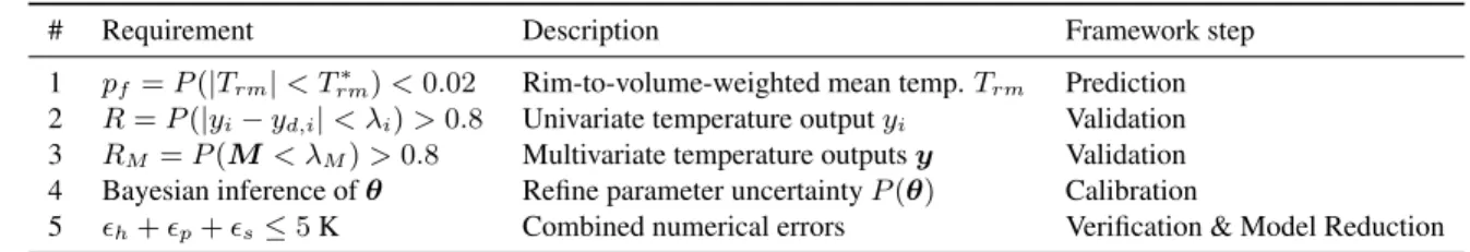
Thus, the model's reliability metric addresses both aspects of requirement 3 and is selected for further expansion in this chapter. Thusλ relates the metric result to engineering units, but unlike the area metric, the model reliability metric's output is a probability value between 0 and 1.
Multivariate validation metrics
- Multivariate model reliability metric
Therefore, this metric was chosen for further extension, along with the univariate area metric and the univariate model reliability metric in Section 6.3, and its mathematical definition is given below. The reliability measure of a multivariate model compares the multivariate distributions of the model and measurements of y using the MD denoted Mj for the measurementsj.
Methodology
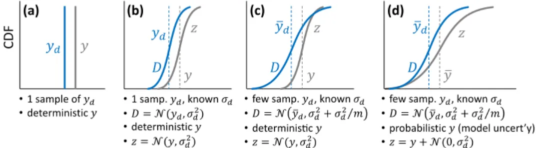
- Distributions used in the validation comparison
- Measurement distribution
- Model output distribution
- Extensions to the area metric
- Limited measurement samples
- Confounding of results between distribution bias and shape
- Extensions to the model reliability metrics
- Limited measurement samples
- Confounding of results between distribution bias and shape
- Setting the accuracy requirement (univariate)
- Setting the accuracy requirement (multivariate)
- Bivariate example of the extended metrics
- Case I univariate metric results for the bivariate model
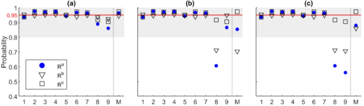
- Case I, II, and III multivariate metric results for the bivariate model
Similar to the area metric, the model reliability metric also suffers from confusion between distributional bias and shape. In previous work, setting the accuracy requirement for the model reliability metric was left to the decision maker.
Application to the heat transfer model
Predicted model outputs
To illustrate the behavior of a specific set of outputs, scatter plots of outputs 8 and 9 are also shown in panels (b) fory and (d) forz. This was addressed by using the predictive distribution, as shown in (d), due to the additional diagonal terms included in Σ.˜.
System response measurements
The standard deviation of the validation data was provided by expert opinion due to inadequate replication (the same value is used for cases DV0−DV3).
Validation assessments and discussion
- Model reliability metrics
- Area metrics
Similar to the results for the model reliability metric, panel (b) shows that the proposed area metric for biasAb8 shows poor model performance and the sign of the metric matches y-yd (as opposed to Aowch is always positive). Contrary to the model reliability metric conclusions in Figure 6.14, the surface metric shows an acceptable result.
Conclusion
This is analogous to using the variance to characterize a distribution in the univariate case. If the distribution of the model output is highly non-normal and 'skewed' (which can be determined by various multivariate normality tests, e.g. [157]), it is possible that the use of covariance is inappropriate or that transformations [158] must be made to the model output before the multivariate metric can be estimated.
Introduction
Background
Several sources of uncertainty were addressed, including input uncertainty, numerical errors (verification and surrogate model), and model parameter uncertainty (quantified via Bayesian calibration). Furthermore, the Bayesian approach can take into account appropriate correlations between sources of uncertainty.
The proposed framework
Model Definition
- Requirements
- Conceptual, mathematical, and computational model
- Uncertainty identification
- Measurements for calibration and validation
For the heat transfer model example, some sources of uncertainty are listed in Table 7.2; the list is not exhaustive but is used to illustrate the framework. The test plan should be developed as part of the VVUQ requirements for the model.
Verification
- Incorporating discretization errors in the VVUQ framework
Discretization error is defined as the difference between the exact solutionf∗and the approximate solution, f∗−fk at mesh level k. The prevailing method in the VVUQ literature for estimating discretization error is Richardson extrapolation (RE Section 3.1.1).
Model Reduction
- Model output dimension reduction
- Model inputs and parameters dimension reduction
- Surrogate model errors
- Aggregated numerical errors versus requirements
However, since this study applies the same transformation to the measurements during calibration, the PCA truncation errors are not required in this step of the framework (section 7.3.4; this approach was also taken for calibration in PC space in [35, 36]). These three variables are set to their original nominal values in the rest of the steps of the VVUQ framework.
Calibration
- Aggregation through Bayesian inference
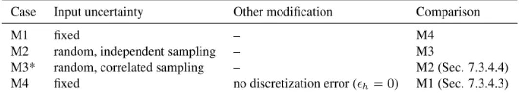
- Model cases for calibration and validation
- The impact of discretization errors on Bayesian inference
- The impact of input uncertainty on Bayesian inference
- A summary of aggregated uncertainty sources
Heat transfer model cases M2 and M3 were defined in Table 7.3 to compare the uncorrelated and correlated sampling approaches, respectively. Another interesting observation is that the correlation between parameters is also affected, eg, the correlation between fwdrouandfrad changes from negative to positive.
Validation
- Model predictions and measurements for validation
- Model validation assessment
- Incorporating the validation assessment into final model predictions
Then, the result of the validation metric is used to expand the posterior parameter uncertainty (Section 7.3.5.3) for QoI prediction. The mean and standard deviation of the parameter distributions in Figure 7.14 are compared in Table 7.8.
Prediction
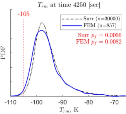
Because the surrogate model runs quickly, many result samples can be produced (3 × 10⁴ in this case), improving the computational efficiency of the error probability calculations. Finally, the surrogate model and FE model predictions are compared at one of the locations used in the validation, P2 (anterior diaphragm, see Figure 7.3).
Conclusion
A better approach to estimate and implement discretization error results for transient errors and combined quantities such as Trm (a spatially averaged quantity) would be useful. First, VVUQ seeks to ensure that the right model is developed for the application - that they are sufficiently "accurate for their intended use".
Summary of contributions
The value of models and measured data to advances in modern engineering cannot be overstated. Third, it fuses models and data (and their sources of uncertainty) to make the best of both and improve decision making.
Future work
Assessing the reliability of complex models: mathematical and statistical foundations of verification, validation and uncertainty quantification. Dynamics model validation using time-domain metrics. Journal of Verification, Validation and Uncertainty Quantification.
Calibration and validation measurement scenarios
Uniform refinement discretization error study settings
Adaptive refinement discretization error study with adaptive error limit settings
Discretization error standard deviation σ h
Calibration parameters
Selected discrepancy function cases and posterior metrics
Definition of bivariate distribution example Cases I-III
Bivariate example validation metric results
Summary of model predictions used in validation
Calibration and validation measurements summary
Representative VVUQ requirements for the heat transfer model
Source of uncertainty and their characterization
Model configurations used to demonstrate calibration and validation of the heat transfer model. 114
Impact of discretization errors on posterior predictions
Impact of input-parameter correlation on parameter posteriors
Impact of input-parameter correlation on posterior predictions
Parameter marginal distributions for posterior and validation-metric-weighted posterior
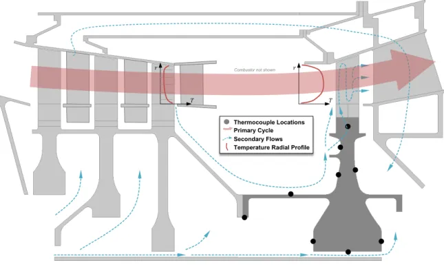
A typical gas turbine engine and its high pressure sub-system
Turbine disc 2D axisymmetric FE model with corresponding measurement locations
Turbine engine square cycle maneuver used for heat transfer model testing
Phenomena identification and ranking table (PIRT)
Illustration of how relative error ϵ h,rel may give a misleading estimate of true error ϵ ∗ h
Turbine disc thermal model discretization error estimation locations
GP fit of temperature for uniformly refined meshes
Discretization error estimator comparison for uniformly refined mesh
GP fit of temperature for adaptively refined meshes
Discretization error estimator comparison of uniformly and adaptively refined mesh
Comparison of uniformly and adaptively refined meshes
Proposed calibration methodology
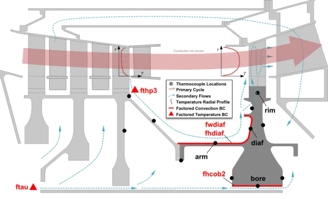
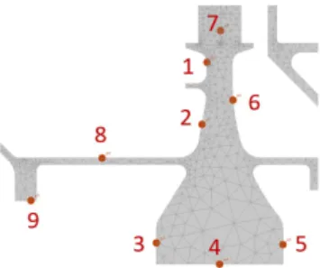
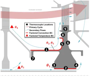
Heat transfer FE model showing selected model parameters and thermocouple locations
Representative FE model transient temperature outputs
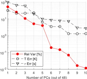
Percentage contribution of PCs to the total variance
Active subspace shadow plots, PC-AS surrogate, and measurements in PC-space
First-order Sobol’ indices compared to active subspace eigenvectors
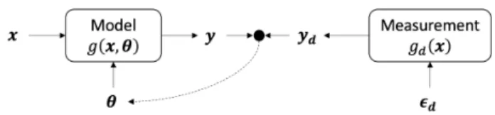
Diagram of the model calibration process
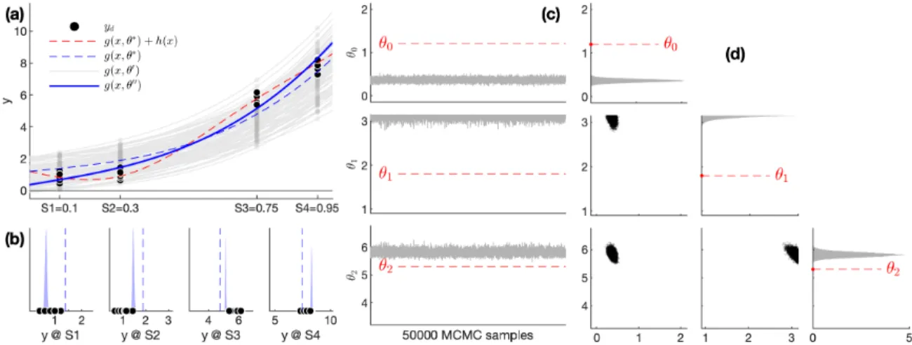
Parameter posterior marginal distributions from the four MCMC cases
Model output posterior predictions
Calibration of the illustrative model without the discrepancy term
Calibration of the illustrative model with a partially identifiable discrepancy term
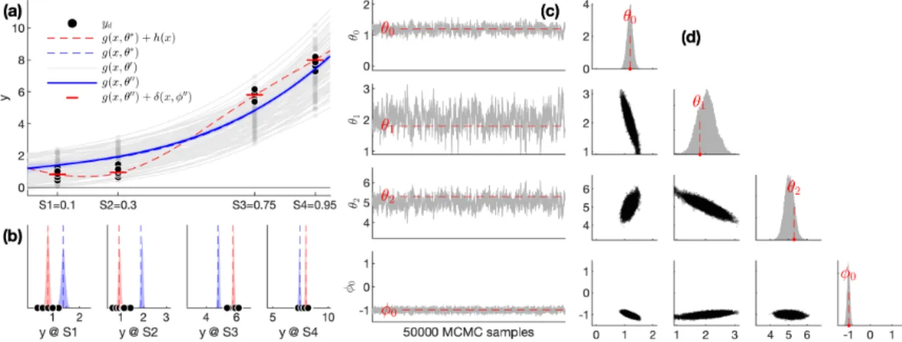
Calibration of the illustrative model with an identifiable discrepancy term
Calibration of the illustrative model in PC space with a non-identifiable discrepancy term
Turbine disc heat transfer model, parameters, and measurement locations
Temperature contours for C 1 and ‘true’ temperature discrepancy
First order Sobol’ indices for each of the first 9 out of 36 PCs
Parameter prior and posterior marginal distributions compared to the true value θ ∗ (Set 1 & 4) . 68
An example histogram distribution of R M
A diagram of the validation process and nomenclature
Scenarios to motivate the use of the expanded distributions D and z in the validation comparison 79
Illustration of the issues when there are limited measurement samples and high correlation in
Illustration of confounding in the model reliability metric
Bivariate example distribution and modified distributions for the extended model reliability
Bivariate example marginal distributions (Case I)
Bivariate example distributions (Case II and III)
Turbine disc 2D axisymmetric FE heat transfer model geometry and output locations
Calibrated model output correlation coefficient and scatter plots
Model reliability metric results for the heat transfer model (two biased outputs)
Model reliability metric results for the heat transfer model (multiple outputs)
Area metric results for the heat transfer model (two biased outputs)
Area metric results for the heat transfer model (multiple outputs)
The uncertainty aggregation framework developed as part of this research
Schematic of the compressor exit air temperature profile
Turbine disc component model showing thermocouple positions
Selected temperature measurements for calibration and validation
Model output to measurement difference (transient)
PCA reconstruction errors
Pareto ordering of maximum Sobol’ indices across all outputs
Impact of discretization errors on parameter posteriors
Impact of input-parameter correlation on parameter posteriors
Sources of uncertainty aggregated through the VVUQ framework
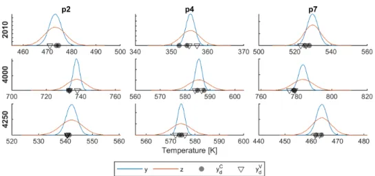
Comparison of posterior prediction distributions of y and z
Computed multivariate model reliability metric distribution for model M3
Univariate and multivariate model reliability metrics for model M3
Parameter marginal distributions for posterior and validation-metric-weighted posterior
Distribution of T rm for the surrogate model and FE model
Prediction of T rm with the full-fidelity heat transfer model
Distribution of temperature at P2 for the surrogate model and FE model