View of THE EFFECT OF MINIMUM WAGES ON EMPLOYMENT IN INDONESIA

Abstract Abstract Abstract Abstract Abstract

Minimum wages have been a major consideration in Indonesia in recent years, as the government has strongly pursued a minimum wage policy. The levels of regional minimum wages have been increased significantly since 1989, and there is a concern that these increases may have slowed employment growth. Therefore, the purpose of this study is to examine the employment effects of minimum wages, using data for 26 provinces, covering the period from 1988 to 1999. The study focuses on different groups of workers within the urban formal sector.

The results of graphical and statistical analysis indicate some support for the conventional theory of the negative employment effects of minimum wages.

THE EFFECT OF MINIMUM WAGES THE EFFECT OF MINIMUM WAGES THE EFFECT OF MINIMUM WAGES THE EFFECT OF MINIMUM WAGES THE EFFECT OF MINIMUM WAGES ON EMPLOYMENT IN INDONESIA ON EMPLOYMENT IN INDONESIA ON EMPLOYMENT IN INDONESIA ON EMPLOYMENT IN INDONESIA ON EMPLOYMENT IN INDONESIA

Leo Sukatrilaksana Leo Sukatrilaksana Leo Sukatrilaksana Leo Sukatrilaksana Leo Sukatrilaksana^*)*)*)*)*)

*) Analis Keuangan Yunior - Biro Perencanaan dan Pengendalian Keuangan Intern

INTRODUCTION INTRODUCTIONINTRODUCTION INTRODUCTIONINTRODUCTION

I

ndonesia has a large labour force, a high unemployment rate and a rapidly expanding labour market. The Indonesian labour market comprises a large proportion of workers who are sensitive to variations in parameters of a minimum wage regime. These groups include females, youth workers and less educated workers. As an illustration, females and youth accounted for 38.4 and 21.3 percent of all labour force participants, respectively, in 1999. Less educated workers accounted for 76.3% of all workers in that year. With these unique economic circumstances, the importance of minimum wages has been a major consideration in the recent years, although minimum wages have been a characteristic of the Indonesia labour market since the early 1970s.

The main reason for the recent importance of minimum wages has been that the government has strongly pursued a minimum wage policy. The levels of minimum wages were increased very significantly, particularly after 1990. This raises concerns whether further large increases in minimum wages will have positive or negative effects on employment. Therefore, the purpose of this study is to evaluate the impact of the increases in minimum wages on various groups of workers in Indonesia.

To provide a framework for this study, theoretical models and the main empirical studies on the links between minimum wages and employment are presented. Some models suggest that increases in the minimum wage that lead to increases in market wages, and which do not correspond to increases in productivity, should have the effect of reducing employment, increasing labour supply and increasing unemployment.

Most of the available empirical evidence on the effects of increases in the minimum wages on employment supports this prediction. On the other hand, the alternative models suggest that the link between minimum wages and employment is not automatically negative, and might even be positive.

This study examines data for 26 provinces, covering the period from 1988 to 1999. A focus is on the specific groups of workers within the urban formal sector, such as females, youth workers, and less educated workers, which have been identified in many previous studies as the groups most vulnerable to changes in minimum wages. Graphical analysis is used to illustrate the possible employment effect in several provinces with the largest urban formal employment. Then, using statistical tools, the study explores a number of alternative models that have been used in the literature for quantifying this employment effect.

The paper is organised as follows. Chapter Two briefly introduces the theoretical framework and the main empirical studies on the links between minimum wages and

employment. Chapter Three illustrates the labour market situation and the practice with respect to minimum wages in Indonesia. Chapter Four investigates the employment effect of the minimum wage in Indonesia by using graphical analysis and statistical tools. Chapter Five summarises this study.

LITERATURE REVIEW LITERATURE REVIEWLITERATURE REVIEW LITERATURE REVIEW LITERATURE REVIEW

2.1.Introduction 2.1.Introduction2.1.Introduction 2.1.Introduction 2.1.Introduction

This chapter briefly introduces the theoretical framework and the main empirical studies on the links between minimum wages and employment. It has two main sections.

The first section examines the predictions of a number of the economic models of minimum wage effects. The first three models consider a competitive labour market in which the available supply of labour is homogeneous. The models suggest that increases in the minimum wage that lead to increases in wages, and which do not correspond to increases in productivity, should have the effect of reducing employment, increasing labour supply and increasing unemployment. This presentation is followed by an outline of alternative models (monopsony, efficiency-wage) which suggest that the link between minimum wages and employment is not automatically negative, and might even be positive.

The second section of this chapter reviews the empirical evidence on the impact of increases in the minimum wage on employment levels. In some studies, the empirical evidence has shown that increases in the minimum wage tend to reduce employment rates.

But other studies claim that minimum wage increases do not necessarily lead to less employment, and may even create more jobs for the unskilled. The main results of these studies will be presented in this section.

2.2. The Theoretical Models 2.2. The Theoretical Models2.2. The Theoretical Models 2.2. The Theoretical Models 2.2. The Theoretical Models

2.2.1. Competitive Labour Market Model 2.2.1. Competitive Labour Market Model2.2.1. Competitive Labour Market Model 2.2.1. Competitive Labour Market Model 2.2.1. Competitive Labour Market Model

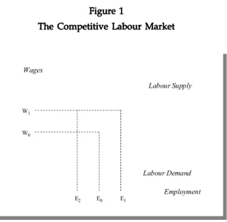
The most basic model of the consequences of minimum wage legislation on employment focuses on a single competitive labour market. In this model, many firms compete for workers while a large number of individuals compete for jobs. Neither a firm nor an individual can affect the equilibrium wage. The available supply of labour is assumed homogeneous. Figure 1 depicts this idealised market.

The amounts of labour supplied and demanded (measured on the horizontal axis) depend on the level of the wage (measured on the vertical axis). The downward-sloping curve represents the marginal productivity of labour. For a given stock of the other factors of production, the contribution to output of each additional worker is assumed to decrease as the total number of workers increases. This curve can be interpreted as a labour demand schedule. The upward-sloping curve represents the alternative earnings of the workers and can be interpreted as a labour supply schedule.

Competitive forces are predicted to operate so that the wage tends towards the equilibrium value, W₀, the wage rate corresponding to the point of intersection of the supply and demand curves. The initial employment is E₀. A minimum wage is simply a wage imposed on the market above the equilibrium wage of W₀. Assume this wage is set at W₁. Following the introduction of the minimum wage of W₁, employment falls to E₂. At this higher wage, more workers will offer themselves for jobs, so labour supply will increase to E₁. Therefore, the effect of the minimum wage is to reduce employment and to create unemployment of E₁-E₂.

This analysis shows there are three major effects of a minimum wage: on employment, on labour supply and on unemployment. There are also effects on the total earnings of labour. All these effects depend on the crucial own-wage elasticities of demand and supply.

These elasticities have been the focus of much of the empirical literature that is reviewed below.

Figure 1 Figure 1 Figure 1 Figure 1 Figure 1

The Competitive Labour Market The Competitive Labour Market The Competitive Labour Market The Competitive Labour Market The Competitive Labour Market

W₀ W₁

E₁

E₂ E₀ Employment

Wages

Labour Supply

Labour Demand W₀

W₁

E₁

E₂ E₀ Employment

Wages

Labour Supply

Labour Demand

2.2.2.

2.2.2.

2.2.2.

2.2.2.

2.2.2.Two-Sector ModelTwo-Sector ModelTwo-Sector ModelTwo-Sector ModelTwo-Sector Model

This model extends the simple model outlined above by considering two sectors of the economy, one being covered by the minimum wage and one that is not covered by the minimum wage. The later sector is termed the uncovered sector.

When the minimum wage is introduced higher than the equilibrium wage in the covered sector, the workers displaced by the minimum wage move to the uncovered sector.¹ This flow of workers will shift the supply curve in the uncovered sector to the right, thereby placing downward pressure on wages in this sector. If we apply the predictions of traditional economic theory, employment in the uncovered sector would increase. It is important to note that unemployment need not result from the minimum wage in this model: rather those who would otherwise have been unemployed in the covered sector can move to the uncovered sector, where the wage can adjust to clear the market.

Brown, Gilroy and Kohen (1982) argued that those displaced from the covered sector do not automatically become employed in the uncovered sector. As wages in the uncovered sector fall, some of those displaced by the minimum wage, as well as a part of those who were originally employed in the uncovered sector, may decide not to work in the uncovered sector because the wage there is less than their reservation wage. Rather they may continue to search for employment in the relatively high wage covered sector. This phenomenon of queuing or “wait unemployment” is analysed in section 2.2.3.

In developed countries, where the coverage of minimum wage appears high, the single- sector model might be appropriate. For developing countries, however, the two-sector model will be more relevant. In these countries only a small share of workers sell their services in a regulated, “formal” sector, subject to a mandated minimum wage. The remainder work in an unregulated, uncovered, “informal” sector, where wages are determined by the market (Packard, 2001, p.4). In the context of Indonesia, for example, the covered and uncovered sectors would refer to a distinction on the basis of employment status. The minimum wage rates and covered sector apply only to employees, while the large proportion of workers who work outside of the wage sector², non-employee workers³, can be considered as members of the uncovered sector. There is also the mobility between these two sectors that is required of the two-sector model: Manning (2000) argued that employees in Indonesia are flexible enough to shift into informal activities as a response to a contraction in labour demand. More detail about the employment status in Indonesia is presented in Chapter 3.

1 This assumes the absence of queuing for covered sector jobs, which is addressed in the next sub-section.

2 In year 2000, workers in uncovered sector comprised 67% of total employment.

3 Non-employee workers are: self-employed workers, employers with permanent workers and unpaid workers.

2.2.3.

2.2.3.2.2.3.

2.2.3.

2.2.3.Two-Sector Model with Queuing for Covered-Sector JobsTwo-Sector Model with Queuing for Covered-Sector JobsTwo-Sector Model with Queuing for Covered-Sector JobsTwo-Sector Model with Queuing for Covered-Sector JobsTwo-Sector Model with Queuing for Covered-Sector Jobs

Mincer (1976) formalised this model as an extension of the two-sector model. It provides the link that relates the effects of a minimum wage to unemployment. Hence Mincer’s approach permits the introduction of a minimum wage to be analysed in terms of the effects on unemployment as well as on employment.

Mincer assumed that workers choose the sector that offers the highest expected wage.

This is given by the probability of obtaining a job in a particular sector times the wage rate in that sector. The covered sector has a (minimum) wage (W_c) greater than that in the uncovered sector (W_u). But the probability of obtaining a covered sector job (P_c) is less than one whereas an uncovered job can be obtained with certainty. Equilibrium in the model requires the equality of the expected wage in each sector. The imposition of a minimum wage that is higher than the equilibrium rate would make a certain amount of “waiting” for jobs in the covered sector worthwhile, thus creating a fixed amount of unemployment (Mincer, 1976, p. S89). Here unemployment is interpreted as queuing for covered-sector jobs.

According to Brown, Gilroy and Kohen (1982), this model makes the overly strong assumption that workers are unlikely to search for covered-sector jobs while employed in the uncovered sector. If the two sectors are geographically separate, this assumption would be realistic. In Indonesia, however, the coverage of the minimum wage depends on employment status (employee or non-employee) and so the markets will not be geographically separate.

However, in many cases it appears as if uncovered sector jobs are employments of last resort for many workers. That is, the workers will work in one sector until circumstances force a change in employment type. They then will seek work in the other sector. Hence, activity (search or employment) in the alternative sectors is separated by a time dimension. This is consistent with the model outlined above.

2.2.4.

2.2.4.2.2.4.

2.2.4.

2.2.4.The Monopsony ModelThe Monopsony ModelThe Monopsony ModelThe Monopsony ModelThe Monopsony Model

In the monopsony labour market, there is effectively only one buyer of labour, so its labour supply schedule is that of the labour market itself. As described in section 2.2.2, this labour supply function relates wage rates to the number of persons seeking employment.

Since the labour supply is a positive function of the wages paid, the firms can attract and retain more workers only if they pay a higher wage.

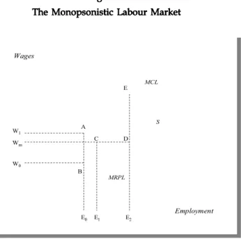
Figure 2 depicts the equilibrium wage and employment in a monopsonistic labour market.

A monopsonist maximizes profit by hiring the amount of labour at E₀, which equates the marginal cost of labour (MCL) to the marginal revenue product of labour (MRPL). Since there is only one firm hiring in this market, E₀ is also total market employment.

Having chosen this level of employment, the monopsonist then offers the wage that will obtain E₀ at minimum cost. This generates an equilibrium wage of W₀. At this wage level, workers are paid less than their marginal value to the firm. This known as monopsonistic exploitation (Fleisher and Kniesner, 1984) and can be measured by the vertical distance AB.

Suppose that a minimum wage equal to W_m is imposed on the labour market. With this minimum wage, the labour supply curve is the kinked line W_mDS. To the left of point D, the supply curve becomes a horizontal line at the value W_m, because workers are prevented from offering their services for less than the minimum wage. To the right of point D, the supply curve follows S, because workers ask a wage rate above the minimum wage level (W_m) in order to supply amounts of labour more than E₂.

The firm’s marginal cost curve becomes horizontal at the minimum wage for amounts of labour less than or equal to E₂. When the quantity of labour exceeds E₂, the marginal cost follows W_mD, then jumps up to E, and follows MCL again. With this new marginal cost of labour schedule, the monopsonist hires the amount of labour that equates its MRPL to its MC.

This occurs at point C and the equilibrium employment and wage become E₁ and W_m. Figure 2

Figure 2Figure 2 Figure 2 Figure 2

The Monopsonistic Labour Market The Monopsonistic Labour Market The Monopsonistic Labour Market The Monopsonistic Labour Market The Monopsonistic Labour Market

W₀ W_m

E₀ E₁ Employment

Wages

S

MRPL MCL

A

B

C D

W₁

E₂ E

W₀ W_m

E₀ E₁ Employment

Wages

S

MRPL MCL

A

B

C D

W₁

E₂ E

The result is that a minimum wage between W₀ and W₁ will increase both the wage and employment above their monopsonistic values, W₀ and E₀. This conclusion can be taken as a possible explanation of the Card-Krueger findings that are reviewed in the empirical literature section below. They suggest that the imposition of the minimum wage can potentially increase employment at affected firms and in the industry as a whole (Card and Krueger, 1994, 1995).

2.2.5.

2.2.5.2.2.5.

2.2.5.

2.2.5.Efficiency-Wage ModelsEfficiency-Wage ModelsEfficiency-Wage ModelsEfficiency-Wage ModelsEfficiency-Wage Models

Traditional neoclassical production theory views wages as determined by prices and labour productivity. However, in reality, compensation has complex incentive properties, and there may be causal links running not just from productivity to wages, but also from wages to productivity.

The central assumption of efficiency-wage models is that there is a benefit as well as a cost to a firm of paying a higher wage (Romer, 1996). According to Mankiw (1997), economists have proposed various theories to explain how wages affect worker productivity. One efficiency-wage theory holds that wages influence nutrition. A higher wage can increase workers’ food consumption, and thereby cause them to be better nourished and more productive. A second efficiency-wage theory holds that high wages reduce labour turnover.

By paying a high wage, a firm reduces the frequency of quits, thereby decreasing the time spent hiring and training new workers. A third theory holds that the higher are wages, the higher the average quality of the firm’s work force. A fourth theory holds that a higher wage can increase workers’ effort in situations where the firm cannot monitor them perfectly. All these theories indicate that the firm operates more efficiently if it pays its workers above the competitive equilibrium wage rate.

These efficiency-wage theories hold that high wages make workers more productive.

As cited by Brown, Gilroy and Kohen (1982), it can be argued that if employers do not minimise costs, there is the possibility that they will respond to a minimum wage increase by raising the productivity of their operation to offset the increase. Wages above the average would increase incentives to work and lead to better economic performance, through lower absenteeism and better adaptation of workers.

2.3. Overview of the Empirical Studies 2.3. Overview of the Empirical Studies2.3. Overview of the Empirical Studies 2.3. Overview of the Empirical Studies 2.3. Overview of the Empirical Studies

The theoretical effects of a minimum wage seem to be ambiguous. The competitive labour market model suggests that the introduction of a minimum wage that raises the wages

of some workers would automatically reduce the employment prospects of that particular category of workers. This simple textbook ‘proof’ of the effect of a minimum wage seems to be what most people have in mind. A survey by Kearl, Pope, Whiting and Wimmer in 1979 showed that 90% of economists working at universities, in government and in the business sector in the United States generally agreed, or agreed with provisions, with the statement that ‘A minimum wage increases unemployment among young and unskilled workers.’ The monopsony and efficiency wage models, however, suggest that the link between wages and employment is not automatically negative, and might be positive. These ambiguous theoretical conclusions are also reflected in the available empirical evidence.

In a comprehensive survey of the empirical literature on minimum wages from the United States, Brown, Gilroy and Kohen (1982) concluded that the empirical evidence was generally in accord with the standard theory. To examine the effects of the minimum wage on teenagers, two sorts of studies were surveyed, namely, time-series studies of teenagers and youth and cross-section studies of teenagers. It is important to note the restriction of the main focus of the Brown et al. (1982) survey: they examine teenagers and youth as these are among the lowest paid workers and so minimum wages are more likely to be effective in these employment markets.⁴

(i) Time-Series Studies of Teenagers and Youth

Time series studies make use of regression techniques to isolate the independent impact of changes over time in minimum wages on employment. Brown et al. (1982) synthesised the results of 25 previous time series studies conducted up to 1981, most of which focused on the teenage labour market. The studies used a single equation model of the type:

Y = f (MW, D, X₁….X_n)

where the dependent variable Y is a measure of labour force status. The independent variables include MW as a measure of the minimum wage, D as an aggregate demand (business cycle) variable to account for changes in the level of economic activity, and X₁….X_n representing a host of other exogenous explanatory variables to control for labour supply, school enrollment, participation in the armed forces, and the like.

The key variable, the minimum wage, has generally been measured by the ratio of the nominal legal minimum wage to average hourly earnings weighted by coverage, the so- called Kaitz Index. The weight applied in this calculation is the number of persons employed in the specific group analysed as a proportion of total employment.

4 An effective minimum wage is one that is imposed above the market clearing wage. A minimum wage imposed below the market clearing wage, as might be the case for older or skilled workers, is said to be ineffective.

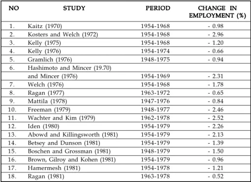
The main summary finding from these time-series econometric studies is that a 10 percent increase in the minimum wage reduces employment among teenagers by 1 percent to 3 percent, holding other factors constant. Table 1 below is adapted from Brown et al.’s (1982) literature review.

1. Kaitz (1970) 1954-1968 - 0.98

2. Kosters and Welch (1972) 1954-1968 - 2.96

3. Kelly (1975) 1954-1968 - 1.20

4. Kelly (1976) 1954-1974 - 0.66

5. Gramlich (1976) 1948-1975 - 0.94

6. Hashimoto and Mincer (19.70)

and Mincer (1976) 1954-1969 - 2.31

7. Welch (1976) 1954-1968 - 1.78

8. Ragan (1977) 1963-1972 - 0.65

9. Mattila (1978) 1947-1976 - 0.84

10. Freeman (1979) 1948-1977 - 2.46

11. Wachter and Kim (1979) 1962-1978 - 2.52

12. Iden (1980) 1954-1979 - 2.26

13. Abowd and Killingsworth (1981) 1954-1979 - 2.13 14. Betsey and Dunson (1981) 1954-1979 - 1.39 15. Boschen and Grossman (1981) 1948-1979 - 1.50 16. Brown, Gilroy and Kohen (1981) 1954-1979 - 0.96

17. Hamermesh (1981) 1954-1978 - 1.21

18. Ragan (1981) 1963-1978 - 0.52

Table 1 Table 1Table 1 Table 1 Table 1

Estimated Impact of a 10 Percent Change in the Minimum Wage Estimated Impact of a 10 Percent Change in the Minimum Wage Estimated Impact of a 10 Percent Change in the Minimum Wage Estimated Impact of a 10 Percent Change in the Minimum Wage Estimated Impact of a 10 Percent Change in the Minimum Wage

on Teenagers 16-19 Years on Teenagers 16-19 Years on Teenagers 16-19 Years on Teenagers 16-19 Years on Teenagers 16-19 Years NO

NONO NO

NO STUDYSTUDYSTUDYSTUDYSTUDY PERIODPERIODPERIODPERIODPERIOD CHANGE INCHANGE INCHANGE INCHANGE INCHANGE IN EMPLOYMENT (%) EMPLOYMENT (%) EMPLOYMENT (%) EMPLOYMENT (%) EMPLOYMENT (%)

Source: Brown, Gilroy and Kohen (1982, pp.498 and 504), Tables 1 and 3

All studies find a negative employment effect for all teenagers together. In addition, the elasticity⁵ signs are almost exclusively negative for the various age-sex-race subgroups considered. The other consistent finding is the unemployment effects of the higher minimum wage are considerably weaker than the disemployment effects because of the withdrawal from the labour force by teenagers in response to a decline in job-prospects. This suggests there is a form of “uncovered” sector for teenagers. It takes the form of the schools sector and non-participation in either the labour market or the schools sector.⁶

5 The elasticity indicates the proportional change in employment, given a proportional change in the minimum wage.

6 In 1999, the number of people aged 15-24 in Indonesia who were not working because they were attending school was 10,733,276 (27.42% of all people aged 15-24) and the number who were not involved in either the labour market or the schools sector was 8,209,731 (20.97% of all people aged 15-24).

(ii) Cross-Section Studies of Teenagers

The cross-section approach involves comparing states or metropolitan areas which differ in the relative importance of their minimum wage. This could be because of variations in the minimum wages across areas (due to State laws) or because of variations in the market wages across areas (due, for instance, to differing levels of economic activity). The survey covered studies that focus on differences in State laws and also those of the effect of the Federal minimum wage on different states.

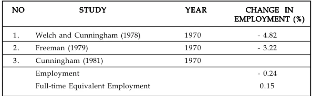
Representative estimates of the employment effects of a 10 percent change in the minimum wage based on these cross-section studies are presented in Table 2 below.

Table 2 Table 2 Table 2 Table 2 Table 2

Estimated Impact of a 10 Percent Change in the Minimum Wage Estimated Impact of a 10 Percent Change in the Minimum Wage Estimated Impact of a 10 Percent Change in the Minimum Wage Estimated Impact of a 10 Percent Change in the Minimum Wage Estimated Impact of a 10 Percent Change in the Minimum Wage

on Teenagers 16-19 Years on Teenagers 16-19 Years on Teenagers 16-19 Years on Teenagers 16-19 Years on Teenagers 16-19 Years

1. Welch and Cunningham (1978) 1970 - 4.82

2. Freeman (1979) 1970 - 3.22

3. Cunningham (1981) 1970

Employment - 0.24

Full-time Equivalent Employment 0.15

NO NONO NO

NO STUDYSTUDYSTUDYSTUDYSTUDY YEARYEARYEARYEARYEAR CHANGE INCHANGE INCHANGE INCHANGE INCHANGE IN EMPLOYMENT (%) EMPLOYMENT (%) EMPLOYMENT (%) EMPLOYMENT (%) EMPLOYMENT (%)

Source: Brown, Gilroy and Kohen (1982, pp.510 and 511), Tables 4 and 5

With a smaller number of studies, empirical studies using cross-sectional data produce a wider range of estimates than the time-series results. Most studies, however, suggest that a 10 percent increase in the minimum wage reduces employment rates among teenagers by about the 1-3 percent range that was found in the time-series studies.

This negative relationship between minimum rates of pay and employment levels established by Brown et al. (1982) in their early survey carries across to more recent studies.

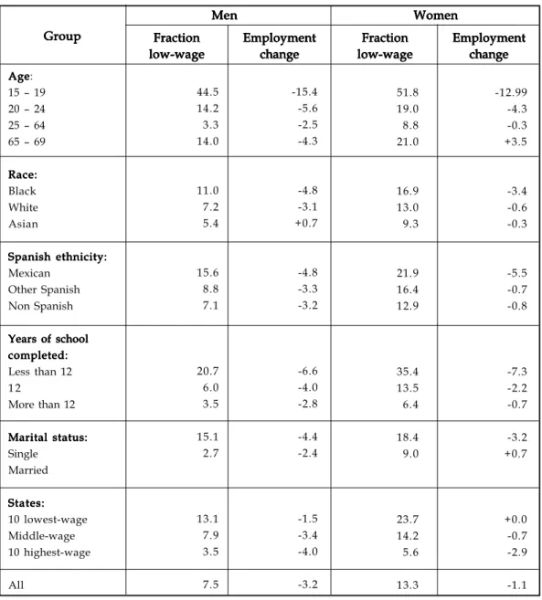
Deere, Murphy and Welch (1995), for example, investigated the employment effects of the more recent increases in the Federal minimum wage in the United States, from $3.35 to $3.80 on April 1, 1990 and then to $4.25 on April 1, 1991. They compared changes in employment rates of high and low-wage populations. Table 3 below lists changes in employment rates relative to the 1989 levels.

Table 3 Table 3 Table 3 Table 3 Table 3

Percentage of Low-wage Workers and Percentage of Low-wage Workers andPercentage of Low-wage Workers and Percentage of Low-wage Workers and Percentage of Low-wage Workers and

the Percentage Change in Employment/Population Ratios the Percentage Change in Employment/Population Ratios the Percentage Change in Employment/Population Ratios the Percentage Change in Employment/Population Ratios the Percentage Change in Employment/Population Ratios

Over Levels for April 1, 1989 – March 31, 1990 Over Levels for April 1, 1989 – March 31, 1990Over Levels for April 1, 1989 – March 31, 1990 Over Levels for April 1, 1989 – March 31, 1990Over Levels for April 1, 1989 – March 31, 1990

Men MenMen Men

Men WomenWomenWomenWomenWomen Group

Group Group Group

Group FractionFractionFractionFractionFraction low-wage low-wagelow-wage low-wage low-wage

Employment Employment Employment Employment Employment

change changechange changechange Fraction

FractionFraction FractionFraction low-wage low-wagelow-wage low-wagelow-wage Employment

EmploymentEmployment Employment Employment

change change change change change Age

Age Age Age Age:

15 – 19 20 – 24 25 – 64 65 – 69 Race:

Race:

Race:

Race:

Race:

Black White Asian

Spanish ethnicity:

Spanish ethnicity:

Spanish ethnicity:

Spanish ethnicity:

Spanish ethnicity:

Mexican Other Spanish Non Spanish Years of school Years of school Years of school Years of school Years of school completed:

completed:

completed:

completed:

completed:

Less than 12 1 2

More than 12 Marital status:

Marital status:

Marital status:

Marital status:

Marital status:

Single Married States:

States:

States:

States:

States:

10 lowest-wage Middle-wage 10 highest-wage All

44.5 14.2 3.3 14.0

11.0 7.2 5.4

15.6 8.8 7.1

20.7 6.0 3.5

15.1 2.7

13.1 7.9 3.5 7.5

-15.4 -5.6 -2.5 -4.3

-4.8 -3.1 +0.7

-4.8 -3.3 -3.2

-6.6 -4.0 -2.8

-4.4 -2.4

-1.5 -3.4 -4.0 -3.2

51.8 19.0 8.8 21.0

16.9 13.0 9.3

21.9 16.4 12.9

35.4 13.5 6.4

18.4 9.0

23.7 14.2 5.6 13.3

-12.99 -4.3 -0.3 +3.5

-3.4 -0.6 -0.3

-5.5 -0.7 -0.8

-7.3 -2.2 -0.7

-3.2 +0.7

+0.0 -0.7 -2.9 -1.1 Source: Deere, Murphy and Welch (1995, p.235), Table 3

The results in Table 3 show that the group with the highest percentage of low-wage workers (in italics) is also the group whose employment shows the greatest drop. For example, the age comparisons show that employment declines are greatest for those aged 15-19, since this group has the highest incidence of low wage workers. Comparisons across racial groups indicate that black workers, the group with the highest percentage of low-wage workers, experienced the largest employment losses. This emphasises the importance of the distinction between effective and ineffective minimum wages. A given minimum rate of pay will be effective for low wage earners only, and hence will have greater impact on the low-skilled sector of the workforce.

It can be seen that there are exceptions to this general finding, namely the gender and geographic splits. The employment rate of women does not fall relative to the rate of men and low-wage employment does not fall more in low-wage states than in higher-wage states.

Deere, Murphy and Welch argued that the minimum wage responses are swamped by the broader trends of increasing labour-market participation of women and by the stronger employment growth in high-wage states than in low-wage states⁷. However, if men and women are viewed separately, the increases in the minimum wage coincide with shifts toward less employment for lower-wage workers within each gender. Similarly for the across-State comparisons that allow for gender effects, where it is found that employment of low-wage workers falls relative to those who typically earn more both in high-wage and low-wage states.

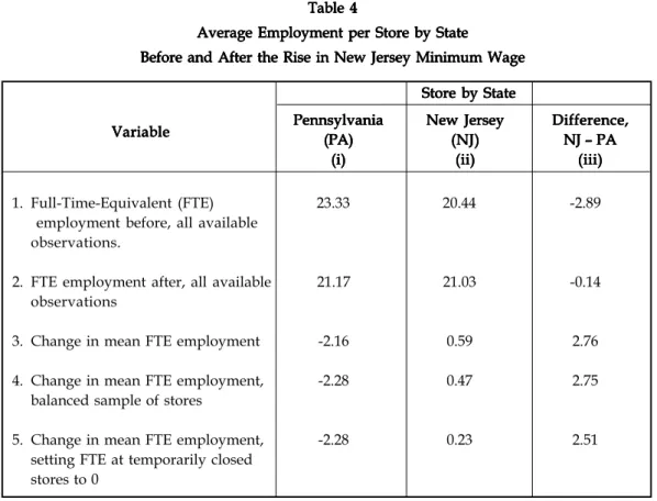
Although most economists believe that, consistent with the evidence reviewed above, increases in the minimum wage reduce employment among workers with little skill and experience, some studies question this conclusion. In September 1994, David Card and Alan Krueger published a study on minimum wages with a focus on the New Jersey minimum wage increase in 1992, where this State raised its minimum wage to $5.05, while the neighbouring State of Pennsylvania kept the Federal rate of $4.25. They examined the fast food industry as the leading employers of low wage earners and an industry that enforces the minimum wage. Their analysis was based on establishment surveys conducted prior to the increase in the minimum wage and after the minimum wage was increased. The first wave of the survey was conducted a little over a month before the scheduled increase in New Jersey’s minimum wage. The second wave was conducted about eight months after the minimum- wage increase. Table 4 summarises the levels and changes in average employment per store by state in their survey.

7 There was an employment expansion in the South and Southwest where wages were lower than in the Northeast, Upper Midwest, and West.

Rows 1 and 2 of the table present data on full-time equivalent employment before (wave 1 of the survey) and after (wave 2 of the survey) the increases in New Jersey’s minimum wage, from all available observations. The changes in average employment between waves 1 and 2 are shown in row 3. An alternative estimate of the change is presented in row 4: in this row, the computation of the change in employment is restricted to the subsample of stores that reported valid employment data in both waves (the balanced subsample). Row 5 presents the average change in employment in the balanced subsample, treating employment at temporarily closed stores in wave 2 as zero, rather than as missing.

After the rise in the minimum wage, stores in New Jersey grew relative to stores in Pennsylvania, with the relative gain being 2.76 FTE employees. When the analysis is restricted to the balanced subsample, the relative change is virtually identical (2.75) to that reported for the full sample, and only slightly smaller (2.51) when employment at temporarily closed stores in wave 2 is treated as zero. Thus this study indicated that employment actually expanded in New Jersey relative to Pennsylvania, where the minimum wage was constant.

Table 4 Table 4Table 4 Table 4 Table 4

Average Employment per Store by State Average Employment per Store by State Average Employment per Store by State Average Employment per Store by State Average Employment per Store by State

Before and After the Rise in New Jersey Minimum Wage Before and After the Rise in New Jersey Minimum WageBefore and After the Rise in New Jersey Minimum Wage Before and After the Rise in New Jersey Minimum Wage Before and After the Rise in New Jersey Minimum Wage

1. Full-Time-Equivalent (FTE) 23.33 20.44 -2.89

employment before, all available observations.

2. FTE employment after, all available 21.17 21.03 -0.14 observations

3. Change in mean FTE employment -2.16 0.59 2.76

4. Change in mean FTE employment, -2.28 0.47 2.75

balanced sample of stores

5. Change in mean FTE employment, -2.28 0.23 2.51

setting FTE at temporarily closed stores to 0

Source: Card and Krueger (1994, p.780), Table 3

Store by State Store by StateStore by State Store by State Store by State

Difference, Difference, Difference, Difference, Difference, NJ – PA NJ – PANJ – PA NJ – PANJ – PA

(iii) (iii)(iii) (iii)(iii) New Jersey

New JerseyNew Jersey New Jersey New Jersey

(NJ) (NJ) (NJ) (NJ) (NJ) (ii) (ii) (ii) (ii) (ii) Pennsylvania

Pennsylvania Pennsylvania Pennsylvania Pennsylvania

(PA) (PA) (PA) (PA) (PA) (i) (i)(i) (i) (i) Variable

VariableVariable Variable Variable

Card and Krueger also compared the low-wage ($4.25 per hour in wave 1) and high- wage ($5.00 or more per hour in wave 1) stores in New Jersey before and after the new minimum wage. This comparison showed that employment expanded at the low-wage stores and contracted at the high-wage stores. This comparison provides a specification test of the validity of the Pennsylvania control group in that the minimum wage is less likely to be effective in the high wage stores in New Jersey and so the employment behaviour in these stores is expected to resemble that in the stores in Pennsylvania.

In some additional research that they conducted using data from other states, Card and Krueger found a positive correlation between a higher minimum wage and employment.

The Card-Krueger study leads us to believe that employers demand more labour as its price rises.

According to Mankiw (1997), one possible explanation of this result is that firms have some market power in the labour market. As shown in section 2.3.4, a monopsonistic firm buys less labour at a lower wage than a competitive firm would. The monopsonistic firm reduces employment in order to depress the wage it has to pay. A minimum wage prevents the monopsonistic firm from following this strategy and so can increase employment.

However, most economists are sceptical of the monopsony explanation, since most firms compete with many other firms for workers.

The Card-Krueger findings have sparked considerable controversy among labour economists and have generated much debate in academic and political circles. Their data have been criticized, and researchers working with better data have shown the result is reversed. A follow-up investigation by Neumark and Wascher (1995) showed that Card and Krueger collected their data incorrectly. In particular, the data collected by Card and Krueger appear to indicate greater employment variation over the eight-month period between their surveys than do payroll data. Moreover, even if the Card-Krueger data were correct, one can argue that their study searched for effects across too few industries and allowed too little time to elapse (Miller, 1995). Richard Berman of the Employment Policies Institute also disagreed with the methodology of the Card and Kruger study. He argued that the analysis should have focused on the number of hours worked instead of the number of employees (Berman, 1998).

In the context of Indonesia, Rama (2001) has attempted to assess the impact of minimum wage policy on the labour market. Based on the results of an econometric analysis of data from 27 provinces for the period from 1988 to 1995, minimum wage policies were shown to have had a modest impact on labour market outcomes. The starting point for his analysis was a basic equation of the type:

where R is an indicator of labour productivity. In his study, Rama used five different indicators of labour productivity: average earnings of urban labourers, average wage in manufacturing, labour costs per worker in large manufacturing, value added per worker in large manufacturing, and GDP per worker excluding oil and gas.

The elasticity in this specification can be calculated as , where is the sample mean of MW_it/R_it and is the sample mean of L_it/N_it. Rama’s results show that the estimated elasticity of employment with respect to minimum wages is statistically significant in only one of the specifications, but it has the same sign (negative) in four of them and is close to zero in the fifth one. Therefore, it can be argued that higher minimum wages reduce wage employment in Indonesia.

Finally, Rama concluded that the doubling of the minimum wage in the first half of the 1990s led to an increase in average wages in the range of 5 to 15 percent, and a decrease in urban wage employment in the range of 0 to 5 percent. However, he suggested that while the disemployment effects appeared to be considerable in small manufacturing firms, employment may have actually increased in large firms. The workers in large firms are the winners from the increases in the minimum wage as their wages increase and there appears to be little risk that they will lose their jobs.

It is important to note that the main focus of Rama’s study was the effects of increases in minimum wages for the whole aggregate of workers. However, as noted above, the impacts of increases in minimum wages on the various groups of workers are not the same, but fall mostly on the groups of workers who are sensitive to variations in parameters of a minimum wage regime. A focus on the specific groups of workers such as females, youth workers, and

it i i it

it

f MW

Z = ( ) + θ + τ + ε

where Z_it is an economic outcome in province i and year t, MW_it is the minimum wage in province i and year t, is a province-specific effect (e.g. infrastructure, natural resources, demography, etc.), is a year-specific effect (e.g. macroeconomic policies, external shocks, the investment climate, etc.) and is a stochastic disturbance.

In examining the impact of minimum wages on employment, Rama used a particular version of the basic equation above. Specifically, the economic outcome focused on by Rama was the ratio of employment to population, that is Z_it = L_it/N_it. The equation to be estimated was:

it i i it it it

it

N b b MW R

L / =

₁

+

₂

( / ) + θ + τ + ε θ

i

τ

i

ε

it

λ µ /

b

2

µ

where and are labour supply and labour demand respectively, represents wages, represents the minimum wage, is a vector of labour supply shifters, is a vector of labour demand shifters, while and are vectors of parameters.

In equilibrium, labour supply is equal to labour demand, and hence:

=

The reduced form solutions for wages and employment are:

less educated workers would have been more informative. This issue becomes a consideration in the more current study by Suryahadi, et al. (2001).

Suryahadi, et al. (2001) use data from 26 provinces, covering the period from 1988 to 1999, to analyse the impact of minimum wages on different groups of workers within the urban formal sector. They defined supply and demand for workers as follows:

X w

m w

l

^S

= α

^S

+ β

^S

+ γ

^S

( ) + θ

^S

X w

m w

l

^D

= α

^D

+ β

^D

+ γ

^D

( ) + θ

^D

l

S

l

^{D w}

m

X Y

γ β

α , , θ

X w

m w

l

^S

= α

^S

+ β

^S

+ γ

^S

( ) + θ

^S

l

^D

= α

^D

+ β

^D

w + γ

^D

m ( w ) + θ

^D

X

X Y

w m

w = Λ

^w

+ Ω

^w

( ) + Π

^w

+ Σ

^w

X Y w

m

l = Λ

^l

+ Ω

^l

( ) + Π

^l

+ Σ

^l

D S

S D w

β β

α α

−

= −

Λ

^w _S^{D S}_D

β β

γ γ

−

= −

Ω

^w _S ^D _D

β β

θ

= −

Π

^w _S ^S _D

β β

θ

−

= − Σ

D S

S D D S l

β β

β α β α

−

−

= −

Λ

^{l S D}_{S D}^{D S}

β β

γ β γ β

−

= −

Ω

^l _S ^{S D}_D

β β

θ β

= −

Π

^l _S ^{D S}_D

β β

θ β

−

= − Σ

where , , , ,

, , ,

The parameters of main interest are and , that is how the minimum wage affects wages and employment. The wage regression results indicate that the impact of minimum wages on average wages across the workforce is mixed. The wages of some workers are pushed up by minimum wages, while the wages of others are depressed by minimum wages.

Ωw Ω^l

The results of employment regression indicate that the elasticity of total employment to the minimum wage is –0.112 and statistically significant. This implies that every 10 percent increase in real minimum wages will result in a 1.1 percent reduction in total employment.

The coefficients for female, youth and less educated workers are also negative and statistically significant. The only group of workers which benefit from the minimum wage are white- collar workers. A 10 percent increase in the real minimum wage is suggested to increase the employment of white-collar workers by 10 percent.

2.4. Conclusion 2.4. Conclusion2.4. Conclusion 2.4. Conclusion 2.4. Conclusion

The theoretical models outlined in this chapter attempt to explain the correlation between the change in minimum wages and employment. According to the competitive models, an increase in the minimum wage that leads to an increase in wages, and which does not correspond to an increase in productivity, would have the effect of reducing employment.

Several criticisms have been advanced against this competitive model. The main one focuses on the fact that the firm is not always a price taker in the labour market (Ghellab, 1998). The alternative models (monopsony and efficiency-wage) suggest that the link between minimum wages and employment is not automatically negative, and might even be positive.

Most of the available empirical evidence on the effects of increases in the minimum wage on employment supports the standard theory that increases in the minimum wage tend to reduce aggregate employment rates and increase unemployment rates.

THE MINIMUM WAGE IN INDONESIA THE MINIMUM WAGE IN INDONESIATHE MINIMUM WAGE IN INDONESIA THE MINIMUM WAGE IN INDONESIA THE MINIMUM WAGE IN INDONESIA 3.1. Introduction

3.1. Introduction3.1. Introduction 3.1. Introduction 3.1. Introduction

The first section of this chapter briefly illustrates the labour market situation in the rapidly changing Indonesian economy. Some key statistics on the Indonesian labour force are presented in this section. The second section describes the practice with respect to minimum wages in Indonesia. This includes an illustration of the minimum wage development and several key problems in its implementation. Finally, we end the chapter with some concluding remarks.

3.2.

3.2.3.2.

3.2.

3.2. The Labour Market SituationThe Labour Market SituationThe Labour Market SituationThe Labour Market SituationThe Labour Market Situation

With a large labour force, a high unemployment rate and a rapidly expanding labour market, Indonesia has fairly unique economic circumstances. Manning (1994, 1998b) describes

The Indonesian labour force grew from 88,186,772 in 1996 to 94,847,178 in 1999 (7.6%

growth). The labour force participation rate was relatively stable between 66 and 68 percent, suggesting that much of the growth in the labour force is due to growth in the population.

The proportion of female and youth labour force also did not change much during the period reviewed. The female labour force varied a little, between 38 and 39 percent of all labour force participants. Similarly, the youth labour force fluctuated between 21 and 23 percent of all labour force participants. It is apparent from the table that there is a large proportion of less educated workers in labour market. However, this proportion decreased from 78.8% in 1996 to 76.3% in 1999.

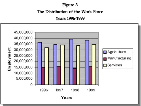
Indonesia is also undergoing rapid structural transformation from agriculture into manufacturing and services. This transformation, however, has been associated with employment patterns that have changed less rapidly than those of output. The reasons behind this are primarily the slow rate of labour movement out of low productivity sectors, especially agriculture, and multiple jobs holding across sectors in the process of the shift out of agriculture (Hill 1996, p. 21). Figure 3 shows the distribution of workers across the main sectors.

It is clearly apparent from Figure 3 that the agricultural sector accounts for the largest share of employment in Indonesia. However, between 1996 and 1997, there was a redistribution of the share of employment away from agriculture and towards the the labour market in Indonesia as having low wages, long working hours, harsh labour management, poor working conditions, utilisation of under legal working age workers, and high rates of informalisation compared with other Asian countries. Table 5 presents some recent labour force characteristics for Indonesia.

T TTTTable 5able 5able 5able 5able 5

The Indonesian Labour Force Characteristics The Indonesian Labour Force CharacteristicsThe Indonesian Labour Force Characteristics The Indonesian Labour Force CharacteristicsThe Indonesian Labour Force Characteristics

Y Y Y Y

Years 1996-1999ears 1996-1999ears 1996-1999ears 1996-1999ears 1996-1999

a: aged 15-24 years old

b: no schooling, unfinished primary, primary, lower secondary

Source: Badan Pusat Statistik /BPS (Central Bureau of Statistics of Indonesia) C H A R A C T E R I S T I C S

C H A R A C T E R I S T I C S C H A R A C T E R I S T I C S C H A R A C T E R I S T I C S

C H A R A C T E R I S T I C S 1 9 9 61 9 9 61 9 9 61 9 9 61 9 9 6 1 9 9 71 9 9 71 9 9 71 9 9 71 9 9 7 1 9 9 81 9 9 81 9 9 81 9 9 81 9 9 8 1 9 9 91 9 9 91 9 9 91 9 9 91 9 9 9

Size of labour force (millions) 88.2 89.6 92.7 94.8

Labour force participation rate (%) 66.9 66.3 66.9 67.2

Female labour force (% of the total labour force) 38.5 38.3 38.8 38.4 Youth labour force (% of the total labour force)^a 22.3 21.5 21.3 21.3 Less educated labour force (% of the total labour force)^b 78.8 77.9 75.8 76.3

manufacturing and services sectors. Thus employment in agriculture fell from 36.5 million (43.5% of total employment) in 1996 to 34.8 million (40.7%) in 1997. During the economic crisis that affected the Asian region in 1997, workers in the manufacturing and services sectors who lost their jobs moved to the rural region and worked on the farms. This phenomenon increased agriculture’s employment to 39.4 million (45.0%) in 1998, while the employment of manufacturing and services decreased from 16.3 million (19.1%) and 34.3 million (40.2%) in 1997 to 14.3 million (16.3%) and 34.0 million (38.8%) in 1998. When the economy started to recover in 1999, employment in the manufacturing and services sectors increased to 15.8 million (17.8%) and 34.6 million (39.0%), respectively.

The impact of the economic crisis on employment in Indonesia was, in fact, less than had been expected. The International Labour Organisation (ILO) had predicted that perhaps as many as 10-14 million people would find themselves without jobs in 1998 (Cameron, 1999). However, the actual employment loss was more likely around 2 million⁸. The key explanations for this better than expected outcome are: the capability of people to find a new job after being cut back from wage employment, and the willingness of employees to accept lower wages, accept shorter work hours and obtain fewer employee benefits (Booth 1999, Manning 2000). Thus, there has been high flexibility in labour market adjustment combined with disobedience of employers toward minimum wage legislation, and low enforcement of

Figure 3 Figure 3Figure 3 Figure 3Figure 3

The Distribution of the Work Force The Distribution of the Work Force The Distribution of the Work Force The Distribution of the Work Force The Distribution of the Work Force

Years 1996-1999 Years 1996-1999 Years 1996-1999 Years 1996-1999 Years 1996-1999

Source: Badan Pusat Statistik /BPS (Central Bureau of Statistics of Indonesia) 0

5,000,000 10,000,000 15,000,000 20,000,000 25,000,000 30,000,000 35,000,000 40,000,000 45,000,000

1996 1997 1998 1999

Ye ars

Employment Agriculture

Manuf acturing Services

8 The number of people who left their jobs between August 1997 and August 1998 is 4,279,000. Of these, 51.1%

or 2,188,000 were finding new jobs, of which 35.2% were in wage-jobs and 64.8% in non-wage jobs.

the legislation that further weakens the bargaining power of workers such that they have no better choice than to accept wages below the legal rate. Therefore, regarding this labour market situation, discussion about the minimum wage in Indonesia and its impact on employment is of considerable interest.

3.3. The Minimum Wage in Practice 3.3. The Minimum Wage in Practice 3.3. The Minimum Wage in Practice 3.3. The Minimum Wage in Practice 3.3. The Minimum Wage in Practice

Minimum Wage Regulation was first introduced in Indonesia in the early era of the New Order Regime⁹, when economic activity was still dominated by home industries, and small and middle sized firms. The objective of this regulation was as a measure that would supposedly protect workers’ interests, raise labour productivity, reduce widespread corruption and stimulate economic activity through a spending effect (Manning, 1993). At that time, the minimum wages were set for construction workers on government projects in Jakarta, and then applied to all workers in general and for other regions.

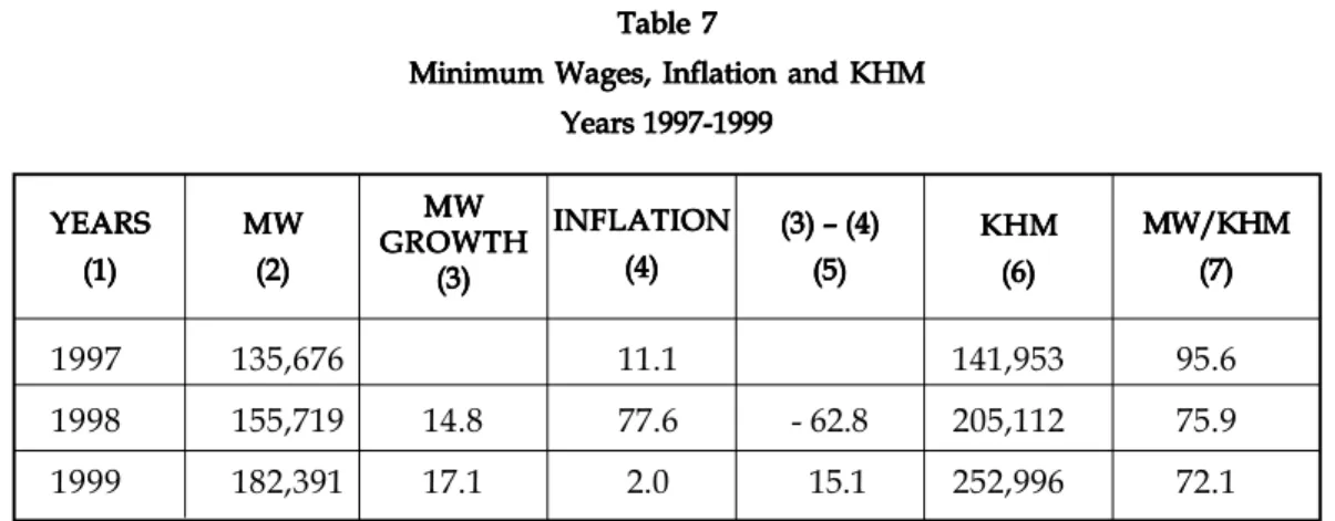
Since the middle of the 1980s, new legislation was established to regularise the haphazard system of minimum wages that had been in force in most regions (Rama, 2001).

The government set the minimum wages with reference to the cost of living, labour market conditions and Minimum Physical Need/KFM (Kebutuhan Fisik Minimum). The KFM is measured by the estimation of a worker’s minimum need in 4 main groups of consumption bundles: food, housing, clothing and a selected other items group. Each group contains a range of items that are considered vital for a single worker to live adequately.

In 1996, the KFM was adjusted with a wider range of consumption bundle and recognised as a Minimum Living Need/KHM (Kebutuhan Hidup Minimum) that represents a higher standard of living than KFM.¹⁰ The KHM bundle consists of 43 items: 11 items in the food group, 19 items in the housing group, 8 items in the clothing group and 5 items in the selected other items group. The improvement of the KHM always becomes a target for policy practitioners in the field of employment management.

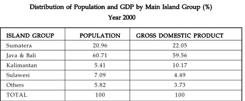
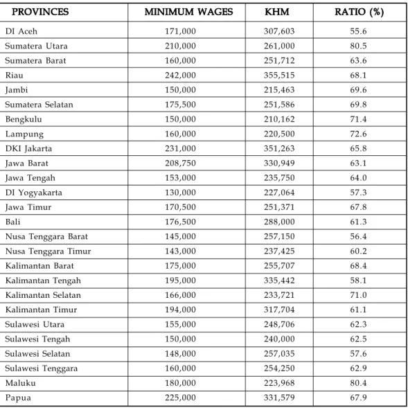
The minimum wages are determined differently among the provinces in Indonesia.

The background behind this policy was the difference of economic structure of the main groups of islands (Inkiriwang, 2001). It can be seen from the data in 2000 that among the groups of islands in Indonesia, Java, Bali and Sumatera have dominated economy activity, accounting for about 80% of Indonesia’s GDP and also of the country’s population. The table below describes the distribution of population and GDP in Indonesia.

9 The New Order Regime from 1966 until 1998, under Soeharto, acted as a ‘state authoritarian corporatist and exclusionary system’ with high state control (Ford, 1999).

10 As cited from “Upah Minimum Sebuah Kajian Tentang Dampaknya Terhadap Penciptaan Lapangan Kerja di Masa Krisis” (Minimum Wage, An Analysis of the Impact of Job Creation during Crisis Era).

In practice, however, until the late 1980s the minimum wage policy was ineffective.

Minimum wages were introduced largely for ‘cosmetic reasons’ (Manning, 1998a, p.116). In large part this was because the government tightly controlled the labour movement by recognising only a single trade union confederation¹¹ (Lambert 1993, Nusantara 1995, Storey 2000). In contrast, in other countries, such as Australia, trade unions are a crucial part of the wage setting process (Miller & Mulvey, 1989). The strong political dictatorship in Indonesia during the New Order Regime prevented unionism from realizing its potential for autonomous action (Hess, 1990) and furthermore the political considerations were frequently more important than economic demands in unions (Hess 1997, Sidik & Iskandaryah 1993, Suwarno

& Elliot 2000). As a result, Manning (1994) pointed out there was little effective direct government or union involvement in the setting of wages.

Moreover, disobedience of employers in Indonesia with respect to the payment of minimum wages, low sanctions imposed on offenders¹² and mild enforcement of legislation by government have all meant that this policy has had little impact on the labour market (Manning 1993, Gall 1998). There was also a lack of regular and genuine inspection, with only 700 labour inspectors to monitor 147,000 companies in 1990, and there are routinely bribes to ignore malpractices (Gall 1998, p. 367). Hess (1997, p. 37) noted that the reason employers often pay less than the minimum wage was the widespread nature of a “patron- client relationship”¹³ in employment relations. This gives employers the opportunity to gain

Table 6 Table 6Table 6 Table 6Table 6

Distribution of Population and GDP by Main Island Group (%) Distribution of Population and GDP by Main Island Group (%)Distribution of Population and GDP by Main Island Group (%) Distribution of Population and GDP by Main Island Group (%) Distribution of Population and GDP by Main Island Group (%)

Year 2000 Year 2000 Year 2000 Year 2000 Year 2000

Source: Badan Pusat Statistik /BPS (Central Bureau of Statistics of Indonesia) ISLAND GROUP

ISLAND GROUP ISLAND GROUP ISLAND GROUP

ISLAND GROUP POPULATIONPOPULATIONPOPULATIONPOPULATIONPOPULATION GROSS DOMESTIC PRODUCTGROSS DOMESTIC PRODUCTGROSS DOMESTIC PRODUCTGROSS DOMESTIC PRODUCTGROSS DOMESTIC PRODUCT

Sumatera 20.96 22.05

Java & Bali 60.71 59.56

Kalimantan 5.41 10.17

Sulawesi 7.09 4.49

Others 5.82 3.73

TOTAL 100 100

11 This union was not designed to represent workers in Indonesia, but it was designed to control their movement (Gall, 1998, p. 366)

12 As cited in Gall (1998, p. 367), penalties for violation of labour laws are too low (three months jail sentence and

$US 55 fine) to have any punitive effect.

13 This relationship is influenced by Javanese culture, with an emphasis on formal behaviour and acceptance of authority (Hess 1997, p. 37).