JDE (Journal of Developing Economies)
https://e-journal.unair.ac.id/JDE/index
DOES FINANCIAL DEVELOPMENT ALLEVIATE POVERTY? EMPIRICAL EVIDENCE FROM INDONESIA
Wahyu Wisnu Wardana*1 Rosa Diwanegara2 Rezza F. Prisandy3
Aminin4 Abdul Rohim5
1,2Department of Economics, Universitas Airlangga, Surabaya, Indonesia
3University of Manchester, Oxford, United Kingdom
4,5STIE PGRI Dewantara Jombang, Jombang, Indonesia
ABSTRACT
This study examines the contribution of financial development to poverty reduction in Indonesia using the autoregressive distributed lag (ARDL) bound testing approach to the cointegration framework. It also employs annual data of several financial development measures such as domestic credit, broad money, and financial development indexes from 1986 to 2018. Our findings suggest that financial development and poverty reduction have a cointegration relationship, regardless of the financial development indicators used.
Furthermore, we find that domestic credit, broad money, financial institution depth, financial market depth, financial market access, and financial market efficiency reduced poverty. It suggests that financial development reduced poverty through its indirect channel, i.e., the economic growth effect.
Keywords: Financial Development, Poverty, Indonesia JEL: G10; G20; I30; O11
To cite this document: Wardana, W. W., Diwanegara, R., Prisandy, R. F., Aminin, & Rohim, A. (2023). Does Financial Development Alleviate Poverty? Empirical Evidence from Indonesia. JDE (Journal of Developing Economies), 8(1), 184-204. https://doi.org/10.20473/jde.v8i1.44648
Introduction
Despite Indonesia’s success in alleviating poverty over the last decades, several challenges remain. The poverty rate decreased considerably from 24 percent in 1999 to 9.8 percent in 2020 (Statistic Indonesia, 2020), but the progress has declined (Majid et al., 2019;
Suryahadi et al., 2012). It dropped from 1.9 percent between the 1970s and 1990s to 0.5 percent between 2002 and 2017 (Purwono et al., 2021; Yusuf, 2018). This is likely to hamper the achievement of Indonesia’s Sustainable Development Goals (SDGs) target, namely, to reduce poverty to 4-4.5 percent by 2030 (Bappenas, 2019). Another challenge is that the country is widely heterogenous, including in the context of poverty. The rates across regions vary, with provinces in the western part of the country showing a lower rate and those in the eastern part showing a higher poverty rate (Sumarto & Bazzi, 2011).
ARTICLE INFO
Received: April 5th, 2023 Revised: May 30th, 2023 Accepted: June 7th, 2023 Online: June 15th, 2023
*Correspondence:
Wahyu Wisnu Wardana
Email: [email protected]
JDE (Journal of Developing Economies) p-ISSN: 2541-1012; e-ISSN: 2528-2018 DOI: 10.20473/jde.v8i1.44648
To tackle the challenges, the government of Indonesia has adopted various policies.
Previously, the anti-poverty policy emphasized a macro and centralized approach (Dartanto
& Nurkholis, 2013). For example, the government subsidized fuel prices as a key policy instrument to achieve social welfare and the rice price ceiling (Perdana, 2014). Currently, the policy is more specifically targeted; for instance, the provision of social assistance for the poor, which includes subsidized rice, conditional cash transfers (CCT), scholarship programs, and subsidized health care (Sumarto & Bazzi, 2011).
Many views that a financial development sector could be an alternative policy to improve the standard of living of people with low incomes (Jeanneney & Kpodar, 2011;
Rewilak, 2017). First, financial development solves financial market imperfections faced by the poor, such as higher lending costs for small borrowers and asymmetric information. Second, it could widen access to formal financing for low-income people to allocate their resources more efficiently (Panjaitan, M.T.H., 2022; Rashid & Intartaglia, 2017). In other words, people with low incomes will be able to save and borrow money to run businesses. Third, financial development may have trickle-down effects on poverty through economic growth channels (Odhiambo, 2010). Improving the financial sector may generate higher economic growth, translating into a lower poverty level.
Nevertheless, some believe the opposite; for example, Rajan and Zingales (2003) and Claessens and Perotti (2007) believed that the improvement in the financial sector, under poor governance, may disproportionally benefit the rich as money would be channeled to the elites who can offer collateral that can ensure a higher probability of repayment success. When a financial system is advancing, the rich might borrow more and leave the poor with lesser access to financing (Odhiambo, 2010; Rashid & Intartaglia, 2017). Such a situation would not help people with low incomes to escape poverty.
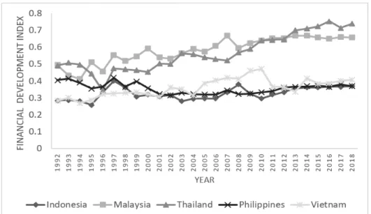
In Indonesia, the long-term trend of financial development shows relatively slow progress. Based on the financial development index (FDI) indicator1, Indonesia’s index was 0.28 in 1992. The figure steadily increased to reach 0.37 in 2018. Compared to the neighboring ASEAN countries such as Malaysia and Thailand (0.66 and 0.74, respectively), Indonesia’s FDI was significantly behind, with a rate similar to Vietnam and the Philippines. Figure 1 depicts the long-term trend of selected ASEAN countries’ FDI from 1992-2018. Considering this, improving financial development in Indonesia is not only feasible but also imperative.
Literature has extensively documented a positive relationship between financial development and economic growth (e.g., Beck & Levine, 2004; Fink et al., 2006; Bist, 2018;
among others), but research on the link between financial development and poverty is limited (Uddin et al., 2014; Majid et al., 2019). Studies in this area have examined the situation in Kenya by Odhiambo (2010) and in Bangladesh by Uddin et al. (2014), compared low, middle, and high-income countries (Dhrifi, 2015), and in selected developing countries (Rashid &
Intartaglia, 2017). However, the studies’ findings have been inconclusive (Odhiambo, 2010;
Uddin et al., 2014)
In Indonesia, Pasuhuk (2018) explored the financial depth and access impact on poverty alleviation using regional data from 2007 to 2015. They confirmed the contribution of financial access and depth to poverty alleviation. Majid et al. (2019) also investigated the same phenomenon by employing the autoregressive distributed lag (ARDL) bound testing model to
1 The International Monetary Fund (IMF) proposes the financial development index to indicate a country’s level of financial development. The index ranges from 0 to 1, with 0 denoting a low financial development level and
annual time series data from 1980 to 2014. They used domestic credit and money supply (M2) as a proxy for the development of the financial sector. Their analysis concluded that both financial development indicators had a long-run relationship with poverty alleviation in Indonesia. However, it is worth noting that the recent study failed to incorporate potential structural breaks stemming from the macroeconomic time series data. It may not be reliable to assume that the long-run relationships among variables are stable (based on the conventional cointegration test). An external shock may shift the variable relationships (Ho & Iyke, 2018).
Uddin et al. (2014) also emphasized that overlooking the time series’ structural breaks may lead to potential bias. Sharma and Syarifuddin (2019) believe that ignoring such a break could influence the analysis’s robustness.
Furthermore, this study only employed two standard quantitative proxies of financial development. It should be noted that financial development is a vast concept with multiple dimensions (World Bank, 2016). Adu et al. (2013) maintained the analysis of financial development contribution is sensitive to the proxy of financial development used.
Source: Svirydzenka (2016)
Figure 1: Index of Financial Development of Selected ASEAN Countries
Thus, this current research aims to assess the causality relationship between financial development, poverty eradication, and economic growth in Indonesia from 1986-2018. This study differs from previous works in several ways. First, this study identifies the structural break in the time series data. Second, the structural break is taken into account in the modeling process. Third, this study enriches the literature by employing financial development indexes proposed by the IMF as an additional indicator of financial development analysis.
The remainder of the paper is organized as follows: the second section reviews the theory on the relationship between financial development and poverty alleviation. The third section lays out the data and methodology of stationary tests and ARDL bound testing approach; the fourth section elaborates on the finding and discussion; and the last section wraps up the discussion.
Literature Review
A financial sector is a set of institutions, instruments, markets, and a legal and regulatory framework that permits transactions to be made by extending credit (World Bank,
2016). Financial sector development is defined as any improvements in the functions, such as savings pooling, funds mobilization, liquidity, trading facilitation, diversification, management of risk, and information generation (World Bank, 2016; Nuru & Gereziher, 2021). According to Schmitz (2010), financial development comprises two essential features: (1) financial deepening, which is the increase of financial market volumes, such as expanding market capitalization, and (2) financial liberalization, which refers to minimal government involvement in the financial market. Financial development is a multifaceted concept (Ho & Iyke, 2018), so measuring it requires variables that could encompass all the attributes (Svirydzenka, 2016).
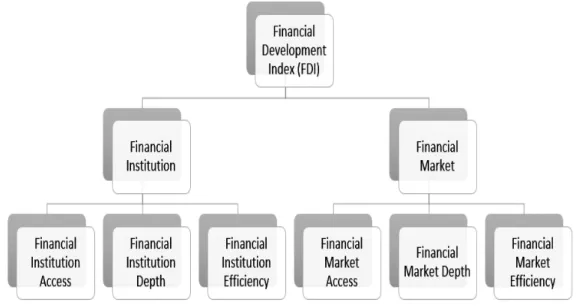
Various proxies have been used to capture financial development, but most studies use the ratio of private sector credit to GDP and the share of stock market capitalization to GDP (Svirydzenka, 2016). IMF proposed a composite index from 0 to 1 called a financial development index (FDI). The index captures financial institutions and market development in terms of depth (size and liquidity), access (individual’s and corporation’s access to financial services), and efficiency (low-cost and sustainable financial services). For example, the depth of financial institutions is measured by the proportion of the private sector’s credit to GDP, the proportion of pension fund assets to GDP, and the ratio of assets of mutual funds to GDP.
In comparison, total units of banks and ATMs represent financial institution access. Financial institutions include banks, mutual funds, insurance companies, and pension funds, and financial markets include stock and bond markets. A high index reflects a high level of financial development and vice versa. A detailed explanation of the methodology and data collection of the index can be found in a study by Svirydzenka (2016). Figure 2 illustrates the component of the financial development index.
Source: Svirydzenka (2016)
Figure 2: The Components of the Financial Development Index
Research on financial development consists of two main strands. The first examines the relationship between financial development and economic growth (Uddin et al., 2014), grounded in the Schumpeterian theory of growth (1911), which claims that a healthy financial system stimulates technological progress through financial services provider for emerging entrepreneurs (Bist, 2018). Past studies have documented this relationship in various scopes, country selections, and time frames (Zhang et al., 2012; Uddin et al., 2014; Arestis, et al., 2001; Samargandi & Kutan, 2016). Most of these studies concur that financial development
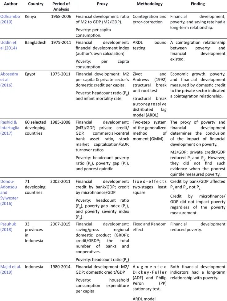
Table 1: Previous Studies on the Relationship between Financial Development and Poverty Alleviation
Author Country Period of
Analysis Proxy Methodology Finding
Odhiambo
(2010) Kenya 1968-2006 Financial development: ratio of M2 to GDP (M2/GDP).
Poverty: per capita consumption.
Cointegration and
error-correction Financial development, poverty, and saving rate had a long-term relationship.
Uddin et
al.(2014) Bangladesh 1975-2011 Financial development:
financial development index (author’s own calculation) Poverty: per capita consumption
ARDL bound
testing A cointegration relationship between poverty and financial development existed.
Abosedra et al.
(2016).
Egypt 1975-2011 Financial development: M2 per capita & private sector’s domestic credit per capita Poverty: headcount ratio (P0) and infant mortality rate.
Zivot and Andrews (1992) structural break unit root test structural break autoregressive distributed lag model (ARDL)
Economic growth, poverty, and financial development measured by domestic credit to the private sector indicated a cointegration relationship.
Rashid &
Intartaglia (2017)
60 selected developing countries
1985-2008 Financial development:
(M3)/GDP, private credit/
GDP, commercial-central bank asset ratio, stock market capitalization/GDP, turnover ratios
Poverty: headcount poverty ratio (P0), poverty gap (P1), and poorest quintile
Two-step system of the generalized method of moment (GMM).
The proxy of poverty and financial development determines the conclusion of the impact of financial development on poverty.
M3/GDP; private credit/GDP reduced P0 and P1. However, they did not find such evidence when the poorest quintile measured poverty.
Donou- Adonsou and Sylwester (2016)
71 developing countries
2002-2011 Financial development:
credit by bank/GDP; credit by microfinance/GDP
Poverty: headcount ratio (P0), poverty gap index (P1), and poverty severity index (P2).
f i x e d - e f f e c t s two-stages least square
Credit by bank/GDP affected P0 and P1, not P2.
Credit by microfinance/
GDP did not impact poverty regardless of the poverty measurement.
Pasuhuk
(2018) 33
provinces in Indonesia
2007-2015 Financial development:
saving/gross regional domestic product (GRDP);
credit/GRDP; the total number of banks and cooperatives.
Poverty: headcount ratio (P0)
Fixed and Random
effect Financial development
reduced poverty.
Majid et al.
(2019) Indonesia 1980-2014. Financial development: M2/
GDP; domestic credit/GDP
Poverty: household consumption expenditure
per capita
A u g m e n t e d D i c k e y - F u l l e r (ADF) and Philip Peron (PP) stationary test.
ARDL model
Both financial development indicators had a long-term relationship with poverty.
The second research strand focuses on financial development’s impact on poverty alleviation, stemming from the hypothesis that sounds financial development addresses market failures, i.e., asymmetric information and high cost of borrowing (Jalilian & Kirkpatrick, 2005). The development of the financial sector also allows poor households to obtain services from formal financial services, i.e., saving and credit activities, enabling them to start and run a new business, increasing saving rate, which raises fund availability for investment activities that stimulate businesses and create more job opportunities (Pasuhuk, 2018). Overall, a well- functioning financial sector could have a trickle-down effect on poverty reduction through an economic growth mechanism (Odhiambo, 2010).
Nevertheless, some argue that financial development does not benefit people with low incomes because, firstly, the advancement may only benefit individuals and enterprises with existing access to financial services (Rashid & Intartaglia, 2017). Secondly, under poor management, the resources may flow to the rich and elites only as they have collateral and powerful political connections (Rajan & Zingales, 2003). Thirdly, any financial instabilities will hurt the chance of reducing poverty (Jeanneney & Kpodar, 2011). Sehrawat and Giri (2018) economic growth and income inequality on poverty in India from 1970 to 2015 by employing the autoregressive distributed lag (ARDL argue that income disparity persists, which is likely to hinder economic growth; not all income segments will benefit from higher economic growth resulting from financial development.
Empirical studies have examined the relationship between financial development and poverty alleviation using various proxies. Selected prior works on the relationship between financial development and poverty are summarized in Table 1.
Data and Research Methods Data Collection
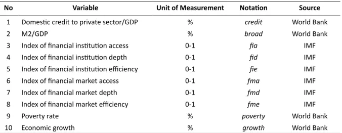
Table 2: Data Description
No Variable Unit of Measurement Notation Source
1 Domestic credit to private sector/GDP % credit World Bank
2 M2/GDP % broad World Bank
3 Index of financial institution access 0-1 fia IMF
4 Index of financial institution depth 0-1 fid IMF
5 Index of financial institution efficiency 0-1 fie IMF
6 Index of financial market access 0-1 fma IMF
7 Index of financial market depth 0-1 fmd IMF
8 Index of financial market efficiency 0-1 fme IMF
9 Poverty rate % poverty World Bank
10 Economic growth % growth World Bank
This study employed the annual time series dataset of Indonesia from 1986 to 2018.
This study used several financial development indicators called: (1) the percentage of domestic credit to GDP; (2) the share of broad money (M2) to GDP; (3) and financial development indexes proposed by IMF: index of financial institution access, index of institution depth, index of institution efficiency, index of financial market access, index of financial market depth, and index of financial market efficiency. Furthermore, this study utilized the variable of poverty, defined as the proportion of people living below $2.15 per day. Meanwhile, the economic growth is the annual growth rate of GDP. Details on the data description are provided in Table
Stationary Test
Several conventional unit root tests examine the stationary properties of time series, such as ADF by Dickey and Fuller (1979) and Ng & Perron (2001). Nevertheless, the unit root tests were unable to test stationary properties in the presence of a structural break. A structural break is a sudden change in time in the time-series dataset (Shrestha & Chowdhury, 2005). To overcome this pitfall, Zivot and Andrew (1992) proposed an alternative unit root test model that allows a single structural break in the time series data at intercept, trend, and both (Uddin et al., 2014). In other words, the Zivot and Andrews unit root test provides information on structural breaks in the time-series dataset. Therefore, the recent study applies ADF and Zivot-Andrews unit root test to check the stationary properties of the variables.
Cointegration Test
The current study uses autoregressive distributed lag (ARDL) bound testing to cointegration technique after stationary test and structural break detection. The strategy provides several advantages over previous cointegration techniques. According to Pesaran et al. (2001), the approach is flexible in terms of the study’s variables’ order of integration. The variables may be integrated in I(1), I(0), or I(1)/(0). The method is also appropriate for small sample sizes, according to Pesaran and Shin (2012). The appropriate lag selection might also prevent variable bias (Pesaran et al., 2001). By following Uddin et al. (2014) and Ho and Lyke (2018), the ARDL bound testing to cointegration’s model specification of this study is provided as follows:
poverty T DUM poverty FD growth
poverty FD growth
t t t
i t i j t j k t k t
k r
j q
i p
0 1 2 3 1 4 1 5 1
1 1
1
3
3 3 3
d d d d d d
d d d n
= + + + + + +
+ + +
- - -
- - -
=
=
=
/ /
/
(1)FD T DUM poverty FD growth
poverty FD growth
t t t
i t i j t j k t k t
k r
j q
i p
0 1 2 3 1 4 1 5 1
1 1
1
3
3 3 3
{ { { { { {
{ { { o
= + + + + + +
+ + +
- - -
- - -
=
=
=
/ /
/
(2)growth T DUM poverty FD growth
poverty FD growth
t t t
i t i j t j k t k t
k r
j q
i p
0 1 2 3 1 4 1 5 1
1 1
1
3
3 3 3
b b b b b b
b b b f
= + + + + + +
+ + +
- - -
- - -
=
=
=
/ /
/
(3)Where denotes financial development proxied by credit, broad, fia, fid, fie, fma, fmd, and fme. Meanwhile, the structural break is considered in the modeling process by adding the variable that represents the dummy variable: 1 when the structural break exists and 0 and vice versa. The notation T indicates the difference operator, and T indicates the time trend.
Furthermore, d { b, , are model parameters, n o, and f, are the error terms (white noise).
The subscript t shows the year, and subscripts i, j, and k represent the order lag. Meanwhile, The notation of summation signs corresponds to the error correction dynamics.
Take an example for equation (1), the null hypothesis that is used to examine the presence of long-term relationship (cointegration) among variables is H0:d3=d4=d5=0 (no cointegration). On the other hand, the alternative hypothesis is H1:d3!d4!d5!0 (cointegration exists). Similar hypothesis testing is applied to equation (2) and equation (3).
The criteria of rejecting or accepting the null hypothesis are based on comparing calculated F statistics with the critical value of F statistics. The null hypothesis is rejected when the estimated
F statistics exceed the upper bound critical value. Conversely, the null hypothesis is accepted when the estimated F statistics are lower than the lower bound critical value. Inconclusive judgment is indicated by approximated F statistics, however, when they fall between the top and lower bounds.
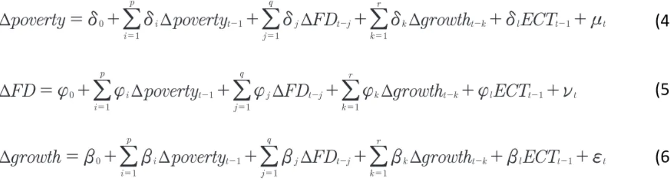
After the confirmation of the existence of cointegration among variables, the next step is to explore the direction of causality among variables that are given in the following form:
poverty i poverty FD growth ECT
i p
t j t j k t k l t t
k r
j q 0
1
1 1
1 1
T =d + dT + d T + d T +d +n
=
- - - -
=
/ /
=/
(4)FD i poverty FD growth ECT
i p
t j t j k t k l t t
k r
j q 0
1
1 1
1 1
T ={ + { T + { T + { T +{ +o
=
- - - -
=
/ /
=/
(5)growth i poverty FD growth ECT
i p
t j t j k t k l t t
k r
j q 0
1
1 1
1 1
T =b + bT + b T + b T +b +f
=
- - - -
=
/ /
=/
(6)Where ECTt-1 indicates the lag value of error obtained from a long-term relationship.
Based on equation (4) - (6), the t statistics of the lagged error correction term that is statistically significant indicates long-term causality. Likewise, F statistics of the first differenced independent variables that are significant indicate the short-run causal relationship’s direction among variables. Additionally, joint short-term and long-run causality between variables could be examined by the joint significance of both the lag value of error (ECTt-1 ) and the first differenced independent variables. Based on this test, there are some potential causal directions of interactions between variables: a unidirectional causality (X to Y and vice versa), a bi-directional causality; and (4) no causal relationship.
Finding and Discussion
The first section of this session explores the stationary properties of the dataset. Two stationary tests are applied: the ADF unit root and Zivot-Andrews unit root tests. Under the ADF unit root test, the decision criteria of the presence of a unit root is based on the value of p-value: a p-value greater than 0.05 indicates the existence of a unit root and vice versa.
Table 3: Unit Root Test by Using ADF
Variable Level 1st Differenced
t-statistic Decision t-statistic Decision
poverty -0.837832 Unit Root -6.718436*** Stationary
growth -3.907*** Stationary - -
credit -4.059*** Stationary - -
broad -4.277** Stationary - -
fia -0.868618 Unit Root -2.655*** Stationary
fid -2.779*** Stationary - -
fie -4.184*** Stationary - -
fma -1.936952 Unit Root -5.836*** Stationary
fmd -2.272315 Unit Root -6.725*** Stationary
fme -3.497*** Stationary - -
Notes: *** p<0.01, ** p<0.05, * p<0.1
Table 3 shows the result of the ADF unit root test. It suggests that four variables, namely poverty, fia, fma, and fmd contain unit roots at level I(0). Thus, the variables should be differenced to avoid unit roots. In other words, the four variables are stationary at the first difference I (1).
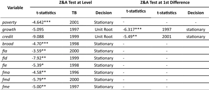
Furthermore, the result of the Zivot-Andrews unit root test is provided in Table 4. The result shows that economic growth and credit variables are the only variables that are not stationary at level I(0). The differentiation of economic growth and credit variable at the first level produced stationary property. Furthermore, the unit root test reveals that most of the variables in the analysis had structural breaks in 1998-1999, when Indonesia experienced a notable economic shock. The economic shock started from the weakening exchange rate, followed by other macroeconomic turbulences. It means that modeling the structural break in the ARDL model is crucial; otherwise, it yields biased estimates.
Table 4: Zivot-Andrews (Z&A) Structural Break Unit Root Test
Variable Z&A Test at Level Z&A Test at 1st Difference
t-statistics TB Decision t-statistics t-statistics Decision
poverty -4.642*** 2001 Stationary - - -
growth -5.095 1997 Unit Root -6.317*** 1997 stationary
credit -9.088 1999 Unit Root -5.49** 2001 stationary
broad -4.70*** 1998 Stationary - -
fia -3.59** 2000 Stationary - -
fid -7.92** 1999 Stationary - -
fie -5.39* 1998 Stationary - -
fma -4.58** 1996 Stationary - -
fmd -5.79** 2000 Stationary - -
fme -5.00** 1997 Stationary - -
Notes: *** p<0.01, ** p<0.05, * p<0.1 and TB is structural break period
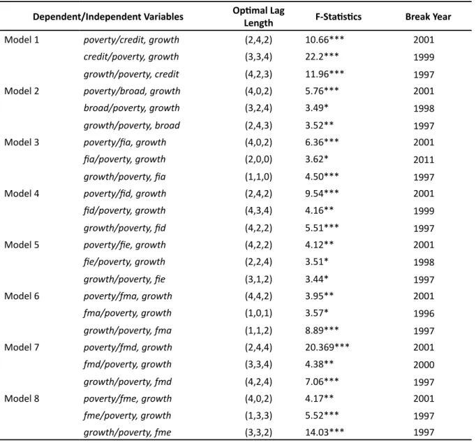
After checking the stationary properties of the variables, the next step is to test the cointegration property among variables. The result of the ARDL bound test cointegration is shown in Table 5. It shows that all ARDL models are statistically significant, at least at the 1%
level, indicating that all variables have a cointegration relationship in the long run. In other words, it implies that the variables move together in the long run. This study aligns with the finding of Majid et al. (2019), which concluded that financial development had a cointegration relationship with poverty, regardless of the measurement of financial development indicators used. This finding contrasts a previous work by Rashid & Intartaglia (2017) that claimed the sensitivity of financial development indicators in poverty-financial development nexus analysis.
Table 6 shows the ARDL estimation in the long run. Six out of eight proxies of financial development significantly lower the poverty rate. Specifically, we documented that private credit (credit), broad money (M2) (broad), financial institution depth (fid), financial market access (fma), financial market depth (fmd), and financial market efficiency (fme) have a significant effect on poverty reduction in Indonesia. By contrast, we do not find such evidence when financial development is proxied by financial institution access (fia) and financial institution efficiency (fie).
Table 5: ARDL Bound Test Cointegration
Dependent/Independent Variables Optimal Lag
Length F-Statistics Break Year
Model 1 poverty/credit, growth (2,4,2) 10.66*** 2001
credit/poverty, growth (3,3,4) 22.2*** 1999
growth/poverty, credit (4,2,3) 11.96*** 1997
Model 2 poverty/broad, growth (4,0,2) 5.76*** 2001
broad/poverty, growth (3,2,4) 3.49* 1998
growth/poverty, broad (2,4,3) 3.52** 1997
Model 3 poverty/fia, growth (4,0,2) 6.36*** 2001
fia/poverty, growth (2,0,0) 3.62* 2011
growth/poverty, fia (1,1,0) 4.50*** 1997
Model 4 poverty/fid, growth (2,4,2) 9.54*** 2001
fid/poverty, growth (4,3,4) 4.16** 1999
growth/poverty, fid (4,2,2) 5.51*** 1997
Model 5 poverty/fie, growth (4,2,2) 4.12** 2001
fie/poverty, growth (2,2,4) 3.51* 1998
growth/poverty, fie (3,1,2) 3.44* 1997
Model 6 poverty/fma, growth (4,4,2) 3.95** 2001
fma/poverty, growth (1,0,1) 3.57* 1996
growth/poverty, fma (1,1,2) 8.89*** 1997
Model 7 poverty/fmd, growth (2,4,4) 20.369*** 2001
fmd/poverty, growth (3,3,4) 4.38** 2000
growth/poverty, fmd (4,2,4) 7.06*** 1997
Model 8 poverty/fme, growth (4,0,2) 4.17** 2001
fme/poverty, growth (1,3,3) 5.52*** 1997
growth/poverty, fme (3,3,2) 14.03*** 1997
Notes: *** p<0.01, ** p<0.05, * p<0.1
The significant impact of the variable of credit, broad, fid, fma, fmd, and fme on poverty reduction demonstrates the importance of financial development. This finding corroborates previous studies by Odhiambo (2010), Uddin et al. (2014), and Abosedra et al. (2016). This finding contrasts with a study by de Haan et al. (2022), who found that financial development does not reduce poverty. According to Zhuang et al.(2009), improvement in financial services’
impact on poverty alleviation runs through two main channels: direct and indirect. The direct channel comes from increased financial access, particularly to people experiencing poverty. Broader access to financial services may lower information and transaction cost, thus allowing poor households to seek external funding for their business. The developing financial sector provides more comprehensive credit access, which provides poor households more opportunities to start or expand their business. Business expansion means higher job creation, allowing poor households to work and earn more income. It is particularly true in developing countries such as Indonesia, where business is predominantly dominated by small, medium-sized enterprises (SMEs) and a significant number of microenterprises. SMEs and microenterprises are labor intensive. Thus, broadening financial credit access to SMEs and microenterprises is expected to increase labor force absorption and raise the incomes
of people experiencing poverty. In addition, better access to financial services allows many households to respond better to adverse economic or health shocks. Therefore, they could mitigate the poverty risk by smoothing their consumption.
Table 6: Long Run ARDL Estimations
Dependent
Variable: Poverty Model 1 Model 2 Model 3 Model 4 Model 5 Model 6 Model 7 Model 8 constant -82.1500 56.698 15.3333 4.4608 6.2382 14.9050 14.2048 10.2645
credit -15.272*** - - - - - - -
broad - -15.275*** - - - - - -
fia - - -89.9176 - - - - -
fid - - - -13.09*** - - - -
fie - - - - -3.9586 - - -
fma - - - - - -12.860* - -
fmd - - - - - - -43.87*** -
fme - - - - - - - -0.7147*
growth 18.6820 -1.55*** 2.9678 2.8762 -0.1195 -0.02*** -8.850*** 4.4245
Diagnostic Test
Adj R-Squared 0.9812 0.9846 0.9826 0.9897 0.9878 0.9854 0.9951 0.9838
LM Test 0.3989 0.4247 0.6333 0.5057 0.5689 0.6819 0.6364 0.2561
Ramsey RESET 0.7556 0.0118 0.0791 0.6382 0.4886 0.2716 0.8369 0.7606 Notes: *** p<0.01, ** p<0.05, * p<0.1
Economic growth is the indirect channel of financial development’s impact on poverty. Levine (2005) believed that sound financial development facilitates growth through 5 mechanisms. The first mechanism is the pooling and mobilization of savings. The process of pooling and mobilization of saving from various savers for profitable investment is relatively costly. Financial services play a role in reducing transaction costs and asymmetric information problems during the savings pooling and mobilization process. This role promotes the effective allocation of financial resources to investments that yield higher returns, boosting economic growth.
Furthermore, effective pooling and mobilization of the saving could facilitate technological innovation, the main driver of sustained economic growth. The second mechanism is providing information. Individual savers face a high cost of obtaining information on the best allocation of their financial resources, restricting the financial capital flow to its best use. Financial development plays a role in reducing information costs through specialization and economies of scale. This process will improve resource allocation and, in turn, raise economic growth. The third mechanism is investment monitoring and exerting corporate governance. Sound financial services monitor firms to use resource allocation efficiently. It also forces managers to maximize the firms’ value and apply good corporate governance. The excellent use of resources and the application of good corporate governance affect savers to finance innovation and production. The fourth mechanism is management diversification. Risk diversification drives technological innovation because funding innovative projects is risky, and a sound financial system can diversify the portfolio in innovative projects, lowering the risk of loss. In other words, the financial system facilitates risk diversification in
services trading facilitation. The financial system serves as a tool for payment for goods and services exchanged in the economy, thus lowering transaction and information costs. This process allows specialization, technological innovation, and economic growth (Bist, 2018;
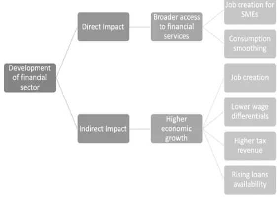
Kheir, 2018). The illustration of the impact of financial development on poverty reduction is shown in Figure 3.
Source: adapted from Zhuang et al. (2009)
Figure 3: The Channel of Effect of Financial Development on Poverty Alleviation The effect of the development of the financial sector on economic growth eventually leads to poverty reduction. Zhuang et al. (2009) argued that there are four potential ways in which economic growth might lower poverty. Higher economic growth is often associated with job creation, especially for poor households. Higher economic growth could also narrow wage inequality between skilled and unskilled labor, benefitting people with low incomes. The subsequent argument is that higher economic growth increases government revenue, allowing the government to spend its fiscal resources on social spending such as health, education, and social protection. This situation helps poor households to increase the quality of their human capital, which often yields poverty alleviation in the long term. Lastly, as capital accumulation rises with the advancing economy, more funds will be available in the loan market for poor households. It allows households to escape poverty.
The significant impact of credit and broad variables on poverty reduction suggest that providing credit is essential. Credit enables firms and entrepreneurs to expand production and introduce new technology in their production process (Impullitti, 2022). Such a process will result in higher economic growth and a lower poverty rate. Similarly, the fid (financial institution depth index) variable is also statistically significant. This variable comprises several indicators, including private-sector credit to GDP; pensions fund assets to GDP; mutual fund assets to GDP; and insurance premiums, life and non-life to GDP. This finding emphasizes the role of credit funds availability in the economy to finance productive activities.
Other significant variables are the financial market depth index (fmd), financial market access index (fma), and financial market efficiency index (fme). The financial market depth index consists of several indicators: capitalization of the stock market to GDP; share of stock traded to GDP; total debt securities of financial corporations to GDP; and total debt securities of non-financial corporations to GDP. In addition, the financial market access index comprised several indicators: percent of market capitalization outside of the top 10 largest companies and the total number of debt issuers (domestic and external, non-financial, and financial corporations). Meanwhile, the index of financial market efficiency is constructed based on the indicator of the turnover ratio of the stock market.
The financial market indicators’ significant impact on poverty reduction demonstrates the importance of the stock market and debt market development. Nevertheless, the development of the stock and debt markets is less likely to be directly linked to poverty reduction. The development of the stock and debt markets is more likely to impact poverty through economic growth channels. In other words, this finding supports the argument that financial development reduces poverty through its indirect channel (Zhuang et al., 2009).
Interestingly, the variable of financial institution access (fia) and financial institution efficiency (fie) did not affect poverty reduction. Several indicators are used to construct the financial institution access index: bank and ATMs units’ availability. Indicators of the lending-deposit spread, return on assets, return on equity, and net interest margin are used to calculate the financial institution efficiency index (fie). The finding suggests that broader access to banking and low cost of financial services does not necessarily lead to poverty reduction. In general, the finding of this current study supports the idea that improving the financial sector lowers poverty through its indirect channel, i.e., economic growth, instead of its direct channel.
It implies that this study opposes the advocates of developing a financial market through broader access to banking.
After the cointegration is found among all models, the following procedure is to check the Granger causality relationship among variables using the VECM method. Table 7 reports the result of the Granger causality test for all eight models. The findings demonstrate that all ECT coefficients are statistically significant and have negative signs. It indicates that the significant ECT’s dependent variables bear the short-run adjustment burden to the long-term relationship among variables. The ECT’s value in all models ranges from about -0.03 to -0.38.
It suggests that the economy requires around 3 – 33 years to correct short-run disequilibrium and achieve long-run equilibrium.
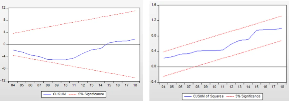
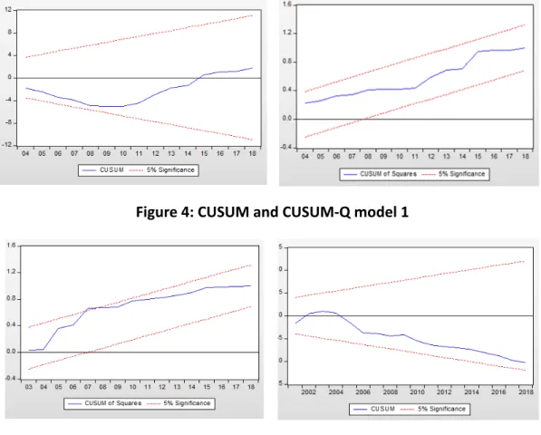
For short-run causality: the findings reveal that poverty and the financial sector (credit, broad, fid, fmd, fma, fme) have a bi-directional relationship. Likewise, economic growth and poverty also have a bi-directional relationship. The results generally align with previous studies that claimed a bi-directional relationship between poverty and financial development (Uddin et al., 2014; Abosedra et al., 2016). Figures 4 to 11 illustrate the plots of the cumulative sum of recursive residuals (CUSUM) and cumulative sum of squared recursive residuals (CUSUMQ) as the test of ARDL’s statistical stability. For instance, Figure 4 shows the CUSUM and CUSUMQ graphs for the ARDL model 1. According to the graphs, the CUSUM and CUSUMQ plots are still within the acceptable bounds of a 5% significant level. It denotes the stability of all ECTs in the predicted ARDL models over short and long-time horizons.
Figure 4: CUSUM and CUSUM-Q model 1
Figure 5: CUSUM and CUSUM-Q model 2
Figure 6: CUSUM and CUSUM-Q model 3
Figure 7: CUSUM and CUSUM-Q model 4
Figure 8: CUSUM and CUSUM-Q model 5
Figure 9: CUSUM and CUSUM-Q model 6
Figure 10: CUSUM and CUSUM-Q model 7
Figure 11: CUSUM and CUSUM-Q model 8
Table 7: VECM Granger Causality Test Dependent VariableIndependent Variables ∑∆POV∑∆GDP∑∆D.Credit∑∆B.Money∑∆FIA∑∆FID∑∆FIE∑∆FMA∑∆FMD∑∆FMEECT(-1) Model 1∆POV-25.51051*0.345591*--------0.042*** ∆GDP4.56031*-3.257139*--------0.054*** ∆D.Credit0.2586**45.215***---------0.104*** Model 2∆POV-5.849**-0.5112**-------0.077* ∆GDP 6.4957**--3.49629*-------0.208*** ∆B.Money8.5390564.245**---------0.3873* Model 3∆POV-39.268***--0.652241------0.129*** ∆GDP2.9337---0.70363------0.038*** ∆FIA0.0446710.205864---------0.18*** Model 4∆POV-25.17771---0.465886-----0.051*** ∆GDP5.237822----4.362953-----0.16*** ∆FID1.35470829.985***---------0.12*** Model 5∆POV-5.415**----1.114472----0.232* ∆GDP 15.13***-----5.9179**----0.081*** ∆FIE8.8634439.978757---------0.028*** Model 6∆POV- 41.40***-----2.901168---0.150*** ∆GDP0.8774------6.041**---0.043*** ∆FMA0.1956950.781234---------0.091*** Model 7∆POV-11.568***------6.105**--0.285** ∆GDP2.729547*-------1.3327*--0.043*** ∆FMD6.98659*1.332726**---------0.113** Model 8 ∆POV-34.875***-------0.1323**-0.16*** ∆GDP2.248975--------2.2489*-0.072*** ∆FME4.0448435.135*** - - - - - - - --0.0052***
Conclusion
This research investigates the long-run relationship between financial development, poverty, and economic growth in Indonesia from 1986 – 2018. This current work is distinct from previous research in several ways: (1) the employment of alternative measures of financial development, namely the financial development index, and (2) the identification and incorporation of structural breaks in the time series data. This current study is expected to enrich the literature on the impact of financial development on poverty reduction.
Our estimation shows that the variable of financial development that is proxied by domestic credit, broad money, financial institution depth index, financial institution access index, financial institution efficiency index, financial market depth index, financial market access index, financial market efficiency index had a cointegration relationship with poverty reduction in Indonesia. Even after considering the issue of a structural break in the analysis, this study supports prior findings regarding the beneficial effect of financial development on eradicating poverty.
Furthermore, the long-run ARDL estimations reveal that six out of eight proxies of financial development reduced poverty. Specifically, domestic credit, broad money, financial institution depth index, financial market depth index, financial market access index, and financial market efficiency index significantly impacted poverty. In contrast, the variable of financial institution access and financial institution efficiency did not impact poverty in Indonesia. The significant role of domestic credit, financial institution depth index, and broad money suggest that credit loan availability is crucial to support real economic activities.
Additionally, financial market indexes’ significant role implies the importance of stock and debt market development in reducing poverty.
Nevertheless, debt and stock market development are less likely to be directly linked to poverty reduction. Thus, we argued that the impact of stock and debt market development on poverty reduction comes from its indirect channel, i.e., the economic growth effect.
Increasing access to financial services does not affect poverty eradication. It means the direct channel on how financial development reduces poverty did not emerge in this context.
The policy implication of this research is as follows. The significant role of several financial development indicators in eradicating poverty calls for the government of Indonesia to diversify the anti-poverty programs. The government may consider financial development as an alternative option to combat poverty in addition to the current strategy (social protection provision). Particularly, the government should push competitive and conducive financial markets to attract firms utilizing financial services. The optimal utilization of financial services for business expansion is expected to create more job opportunities and raise incomes.
Lastly, this research is a macro-based study; hence future research may explore the impact of financial development on poverty from a micro standpoint.
Declarations
Declarations include Conflict of Interest, Availability of Data and Materials, Author’s Contribution, Funding Sources, and Acknowledgements.
Conflict of Interests
There are no conflicts of interest.
Availability of Data and Materials Data is available upon request.
Author’s Contribution
Wahyu Wisnu Wardana: research conceptualization, data analysis, writing the manuscript. Rosa Diwanegara: data collection and analysis. Rezza F. Prisandy: Literature review and writing the manuscript. Aminin: Writing manuscript. Abdul Rohim: Writing manuscript.
Funding Sources
No funding was received to conduct this research.
Acknowledgments -
References
Abosedra, S., Shahbaz, M., & Nawaz, K. (2016). Modeling causality between financial deepening and poverty reduction in Egypt. Social Indicators Research, 126(3), 955–969. https://doi.
org/10.1007/s11205-015-0929-2
Adu, G., Marbuah, G., & Mensah, J. T. (2013). Financial development and economic growth in Ghana: Does the measure of financial development matter? Review of Development Finance, 3(4), 192–203. https://doi.org/10.1016/j.rdf.2013.11.001
Andrew, Z. and. (1992). Further evidence on the great crash, oil-price shock, and the unit-root hyphothesis. Journal of Business Economics Statistic. https://
users.ssc.wisc.edu/~bhansen/718/ZivotAndrews1992.pdf.https://doi.
org/10.1198/073500102753410372
Arestis, P., Demetriades, P. O., & Luintel, K. B. (2001). Financial development and economic growth: the role of stock markets. Journal of money, credit and banking, 16-41. https://
doi.org/10.2307/2673870
Bappenas. (2019). Roadmap of SDGs Indonesia : A Hihglight. 27–36. https://www.unicef.
org/indonesia/sites/unicef.org.indonesia/files/2019-07/ROADMAP%20OF%20SDGs%20 INDONESIA_final%20draft.pdf
Beck, T., & Levine, R. (2004). Stock markets, banks, and growth: Panel evidence. Journal of Banking and Finance, 28(3), 423–442. https://doi.org/10.1016/S0378-4266(02)00408-9 Bist, J. P. (2018). Financial development and economic growth: Evidence from a panel of 16
African and non-African low-income countries. Cogent Economics and Finance, 6(1).
https://doi.org/10.1080/23322039.2018.1449780
Claessens, S., & Perotti, E. (2007). Finance and inequality: Channels and evidence. Journal of Comparative Economics, 35(4), 748–773. https://doi.org/10.1016/j.jce.2007.07.002 Dartanto, T., & Nurkholis. (2013). The determinants of poverty dynamics in Indonesia: evidence
from panel data. Bulletin of Indonesian Economic Studies, 49(1), 61–84. https://doi.org/
10.1080/00074918.2013.772939
de Haan, J., Pleninger, R., & Sturm, J. E. (2022). Does financial development reduce the
poverty gap? Social Indicators Research, 161(1), 0–27. https://doi.org/10.1007/s11205- 021-02705-8
Dhrifi, A. (2015). Financial development and the “Growth-inequality-poverty” triangle.
Journal of the Knowledge Economy, 6(4), 1163–1176. https://doi.org/10.1007/s13132- 014-0200-0
Dickey, D. A., & Fuller, W. A. (1979). Distribution of the estimators for autoregressive time series with a unit root. Journal of the American statistical association, 74(366a), 427-431.
https://doi.org/10.2307/2286348
Donou-Adonsou, F., & Sylwester, K. (2016). Financial development and poverty reduction in developing countries: New evidence from banks and microfinance institutions. Review of Development Finance, 6(1), 82–90. https://doi.org/10.1016/j.rdf.2016.06.002
Fink, G., Haiss, P., & Vukšić, G. (2006). Importance of financial sectors for growth in accession countries. Financial Development, Integration and Stability, 154–185. https://doi.
org/10.4337/9781847203038.00019
Ho, S. Y., & Iyke, B. N. (2018). Finance-growth-poverty nexus: a re-assessment of the trickle- down hypothesis in China. Economic Change and Restructuring, 51(3), 221–247. https://
doi.org/10.1007/s10644-017-9203-8
Impullitti, G. (2022). Credit constraints, selection and productivity growth. Economic Modelling, 111, 105797. https://doi.org/10.1016/j.econmod.2022.105797
Jalilian, H., & Kirkpatrick, C. (2005). Does financial development contribute to poverty reduction? Journal of Development Studies, 41(4), 636–656. https://doi.
org/10.1080/00220380500092754
Jeanneney, S. G., & Kpodar, K. (2011). Financial development and poverty reduction: Can there be a benefit without a cost? Journal of Development Studies, 47(1), 143–163. https://doi.
org/10.1080/00220388.2010.506918
Kheir, V. B. (2018). The nexus between financial development and poverty reduction in Egypt.
Review of Economics and Political Science, 3(2), 40–55. https://doi.org/10.1108/REPS- 07-2018-003
Levine, R. (2005). Chapter 12 finance and growth: Theory and evidence. Handbook of Economic Growth, 1(SUPPL. PART A), 865–934. https://doi.org/10.1016/S1574-0684(05)01012-9 Majid, M. S. A., Dewi, S., Aliasuddin, & Kassim, S. H. (2019). Does financial development reduce
poverty? Empirical evidence from Indonesia. Journal of the Knowledge Economy, 10(3), 1019–1036. https://doi.org/10.1007/s13132-017-0509-6
Ng, S., & Perron, P. (2001). Lag length selection and the construction of unit root tests with good size and power. Econometrica, 69(6), 1519-1554. https://doi.org/10.1111/1468- 0262.00256
Nuru, N. Y., & Gereziher, H. Y. (2021). The impacts of public expenditure innovations on real exchange rate volatility in South Africa (No. 2021/72). WIDER Working Paper.
doi:10.35188/UNU-WIDER/2021/010-8
Odhiambo, N. M. (2010). Is financial development a spur to poverty reduction?
org/10.1108/01443581011061311
Panjaitan, M. T. H. . (2022). Does good financial development attract tourists? Evidence from ASEAN countries. JDE (Journal of Developing Economies), 7(2), 342–353. https://doi.
org/10.20473/jde.v7i2.37433
Pasuhuk, P. M. (2018). Contribution of financial depth and financial access to poverty reduction in Indonesia. Buletin Ekonomi Moneter Dan Perbankan, 21(1), 95–122. https://
doi.org/10.21098/bemp.v21i1.892
Perdana, A. A. (2014). The future of social welfare programs in Indonesia: from fossil-fuel subsidies to better social protection. Winnipeg, Manitoba: International Institute for Sustainable Development.
Pesaran, M. H., & Shin, Y. (2012). An autoregressive distributed-lag modelling approach to cointegration analysis. Econometrics and Economic Theory in the 20th Century, 371–413.
https://doi.org/10.1017/ccol521633230.011
Pesaran, M. H., Shin, Y., & Smith, R. J. (2001). Bounds testing approaches to the analysis of level relationships. Journal of Applied Econometrics, 16(3), 289–326. https://doi.org/10.1002/
jae.616
Phillips, P. C. B., & Perron, P. (1988). Testing for a unit root in time series regression. Biometrika, 75(2), 335–346. https://doi.org/10.1093/biomet/75.2.335
Purwono, R., Wardana, W. W., Haryanto, T., & Khoerul Mubin, M. (2021). Poverty dynamics in Indonesia: empirical evidence from three main approaches. World Development Perspectives, 23, 100346. https://doi.org/10.1016/j.wdp.2021.100346
Rajan, R. G., & Zingales, L. (2003). The great reversals: The politics of financial development in the twentieth century. Journal of Financial Economics, 69(1), 5–50. https://doi.
org/10.1016/S0304-405X(03)00125-9
Rashid, A., & Intartaglia, M. (2017). Financial development – does it lessen poverty? Journal of Economic Studies, 44(1), 69–86. https://doi.org/10.1108/JES-06-2015-0111
Rewilak, J. (2017). The role of financial development in poverty reduction. Review of Development Finance, 7(2), 169–176. https://doi.org/10.1016/j.rdf.2017.10.001
Samargandi, N., & Kutan, A. M. (2016). Private credit spillovers and economic growth: Evidence from BRICS countries. Journal of International Financial Markets, Institutions and Money, 44, 56–84. https://doi.org/10.1016/j.intfin.2016.04.010
Schmitz, M. (2010). Financial markets and international risk sharing. Open Economies Review, 21(3), 413–431. https://doi.org/10.1007/s11079-008-9100-x
Sehrawat, M., & Giri, A. K. (2018). The impact of financial development, economic growth, income inequality on poverty: evidence from India. Empirical Economics, 55(4), 1585–
1602. https://doi.org/10.1007/s00181-017-1321-7
Sharma, S. S., & Syarifuddin, F. (2019). Determinants of Indonesia’s income velocity of money.
Buletin Ekonomi Moneter dan Perbankan, 21(3), 323–342. https://doi.org/10.21098/
bemp.v21i3.1006
Shrestha, M., & Chowdhury, K. (2005). A sequential procedure for testing unit roots in the