S8dhan& Vol. 15, Part 2, September 1990, pp. 73-t03. © Printed in India.
Breakage and coalescence of drops in turbulent stirred dispersions
D K R NAMBIAR, R KUMAR* and K S GANDHI
Department of Chemical Engineering, *and also Jawaharlal Nehru Centre for Advanced Scientific Research, Indian Institute of Science, Bangalore 560012, India
MS received 4 September 1990
Abstract. The various existing models for predicting the maximum stable drop diameter dma x in turbulent stirred dispersions have been reviewed.
Variations in the basic framework dictated by additional complexities such as the presence of drag reducing agents in the continuous phase, or viscoelasticity of the dispersed phase have been outlined. Drop breakage in the presence of surfactants in the continuous phase has also been analysed. Finally, the various approaches to obtaining expressions for the breakage and coalescence frequencies, needed to solve the population balance equation for the number density function of the dispersed phase droplets, have been discussed.
Keywords. Drop breakage; coalescence of drops; stirred vessels; size distribution of drops in stirred vessels; turbulence; maximum stable drop diameter; breakage frequency; coalescence frequency.
! Introduction
Mechanical agitation is a commonly employed method for generating and maintaining a dispersion of one liquid phase in another. Two approaches are available to quantitatively predict the rates of heat and mass transport in such dispersions. The commonly used approach considers all the drops existing in the vessel to be identical in size, and as having identical properties. Thus, an average drop size, an average transfer coefficient and a uniform driving force are used. The average drop size, called the "Sauter mean diameter', d32, is defined in such a way that the total surface area available for transport is conserved. The area per unit volume of the dispersion can then be calculated by
a = 6~/d32. (1)
As d32 does not have a theoretical basis which can be exploited for its prediction,
A list of symbols is given at the end of the paper
73
attempts have been made to predict dmax, the diameter of the largest drop that cannot be further broken in the vicinity of the impeller. The value of d32 is then determined from dmax by dividing it with an empirically obtained factor (lying between 1.5 and 1"6 for most systems). The main difficulty with the averaging method is that it bypasses the fact that most transport processes can vary widely from drop to drop. Schumpe
& Deckwer (1980) have shown that averaging can lead to results significantly different from those obtained experimentally. Further, the mixing of the dispersed phase depends on coalescence and breakage of drops which occur at finite rates, whereas the averaging technique assumes infinite rates of coalescence and breakage. A prelude to such work that accounts for these processes must be the description of just the coalescence and breakage processes. Thus attempts are being made to consider individual drop sizes along with their rates of coalescence and breakage to obtain a more realistic description of a stirred dispersion. This is achieved through the frame work of population balance equations (Hulburt & Katz 1964).
The number balance equation for the dispersed phase droplets can be written as:
dn(v, t) _ ~ F(v')n(v', t)~(v, v')?(v')dv' -
~t
A
- F(v)n(v, t) + q(v - v', v')n(v - v', t)n(v', t)do' -
- f o q ( V , v ' ) n ( v , t ) n ( v ' , t ) d v ' + N o ( o , t ) - n ( v , t ) f o ( v ). (2) The first term on the right hand side of the above equation represents the rate of formation of drops of size v due to breakage of drops of size larger than v. The second term denotes the rate of disappearance of drops of volume v due to breakage. The third term signifies the rate of formation of drops of size v due to coalescence between droplets of volume v - v' and v'. The fourth term describes the rate at which drops of volume v are lost due to their coalescence with other drops. The fifth and sixth terms denote the input and escape rates of the drops of volume v. The left hand side of the equation is the rate of accumulation of drops of volume v, as a result of their birth and death due to breakage and coalescence, as well as feed and escape.
The fifth and sixth terms of (2) vanish for a batch system. In order to solve the population balance equation, a knowledge of the breakage frequency, the probability distribution of the size of the daughter droplets, the number of fragments formed upon breakage, and the coalescence frequency are needed. Separate models are required to obtain expressions for various terms involving breakage and coalescence of drops, which are then incorporated in the population balance equation.
A brief outline of the paper is given below. As the knowledge of dma~ is important for the evaluatign of both d32 and breakage frequency, the basic framework required for its prediction is first discussed along with the information about turbulence in stirred vessels. Based on this framework, models for predicting dma~'for rheologicaUy complex dispersed phases and for situations where surfactants or drag reducing agents are added to the continuous phase are then discussed. All these models assume that a drop invariably breaks into two equal drops. It is then shown that the drops can break into two unequal parts. The conditions under which this could happen are then modelled. The breakage frequency models based on equal and unequal breakage
Breakage and coalescence of drops 75 follow in natural sequence. It is shown that the unequal breakage model, along with the energy cascade theory of distribution of energy into eddies of different length scales, can predict not only the breakage frequency but also the drop size distribution of the daughter droplets. The drop size distribution for a breakage controlled situation is then obtained by using a simplified population balance equation. Coalescence frequency is the product of collision frequency and coalescence efficiency. Models for both these are described. At the end of each major section, a short discussion is presented regarding the weaknesses in our present understanding and the problems to be solved by further work.
2. Drop breakage in stirred vessels
Understanding of the breakage phenomenon is necessary both for the prediction of dma x (which in turn is used for determining d32 ) and for obtaining expressions for breakage related terms like breakage frequency to be used in the population balance equations.
Most of the models available up to this time assume that breakage primarily occurs because of the pressure difference operating across the drop due to turbulent velocity fluctuations. The drop experiencing these stresses tends to deform away from the spherical shape and hence experiences a shape restoring stress due to interfacial tension. Further, if the flow within the drop is assumed to be laminar, there will be a viscous stress retarding the rate of deformation. The deformation of the drop is three-dimensional. Unfortunately we do not yet have a clear picture of the three- dimensional flow field in the vicinity of the drop. Hence one-dimensional models, which capture the gross features of the breakage phenomenon but bypass the detailed flow field, are being developed at this stage.
2.1 Turbulence characteristics of stirred vessels
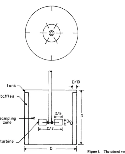
A stirred vessel along with the Rushton impeller and baffles is shown in figure 1.
Different types of impellers are employed in stirred vessels, depending on the flow characteristics desired. The Rushton turbine impeller is normally used for dispersions, whereas other types of impellers are employed when high circulation rates are desired.
Several workers (Nishikawa et al 1976; Okamoto et al 1981; Benyad et al 1985;
Bujalski et al 1987; Costes & Coudrec 1988a, b) have reported data on turbulence intensities, autocorrelation functions, turbulence scales, energy spectra, and turbulence energy dissipation rates in stirred vessels. In general it is found that 60~ of the energy transmitted to the liquid by the impeller is dissipated in the region around the impeller;
the volume of this region being only about 109/o of the total volume. Thus the energy dissipation rates in this zone are nearly fifteen times as large as that in the region away from the impeller. It is observed that the energy spectra show a - 5/3 slope in the higher frequency range and this has been the basis for assuming that the turbulence in the impeller zone is homogeneous and isotropic. This facilitates the application of the energy cascade theory to estimate the energy contained in the eddies in the inertial subrange, the size range occupied by the drops produced in the stirred vessels.
The above picture however shows that hydrodynamics in a stirred vessel is quite complex with zones of high turbulence intensity as well as zones of low turbulence
tank--%
baffles \
sampling --
z o n e
turbine _ ~
L I"
I DI8
D
DIIO
-T
D
J
Figure I. The stirred vessel.
intensity where viscous shear could be more important. This could be of relevance to both breakage as well as coalescence phenomena since these depend crucially on the type of flow field in which they take place.
The above reported measurements are in homogeneous media. A dispersion is however a heterogeneous system and as the volume occupied by the dispersed phase increases, the turbulence characteristics are bound to be altered. Due to the experimental difficulties involved, measurements on such systems have so far not been reported and this imposes serious limitations on theoretical developments in dispersions with high volume fractions.
For all the analyses available, it is assumed that the isotropic turbulence theory can be used. This is justified to some extent as breakage is likely to occur in the zone surrounding the impeller where the turbulence intensity is very high. Experimental measurements also show that the drop size increases as we move farther away from the impeller.
Turbulence has been associated with the presence of eddies, often visualized as simultaneously rotating and elongating fluid elements. The application of turbulent stress on the drop is referred to as drop-eddy interaction, which lasts till the lifetime of the eddy. The largest eddy present in the vessel cannot ~ larger than the blade size of the impeller. The eddy size decreases thereby resulting in an energy cascade.
Breakaye and coalescence of drops 77 Eventually the energy of the eddies gets dissipated as heat when the eddy sizes reach the Kolmogorov scale. As the eddy size decreases, the energy associated with the eddy as well as its lifetime decrease. If a drop interacts with a much larger eddy it simply gets convected. As the eddy size becomes smaller and nearly equal to the drop size it is able to deform the drop. As both the lifetime and energy of a large eddy are high, and the restoring stress for a big drop is small, the large eddy is able to break a drop of equal size. With decreasing drop and eddy sizes, the lifetime and energy of the eddy will decrease whereas the shape-restoring interfacial tension stress will increase. A drop size is finally reached which cannot be broken by the eddy in its lifetime. This drop size is the maximum possible one existing near the impeller and is referred to as dma,. This conceptual picture can form the basis of predictive theories for dma~. It is assumed in all these models that the same stress remains on a drop for the lifetime of the eddy in spite of the fact that the drop is moving.
It has been found that the Sauter mean diameter is approximately 60~,~ of dma x.
Although this relationship can be wrong by about 30~o in case of very viscous dispersed phases, the conceptual convenience with which theories can be developed for dmax has led several investigators to focus on predicting dma x.
2.2 Models for the prediction of dma x
2.2a Dispersed phases of low viscosity: Kolmogorov (1949) and Hinze (1955) were the very first to develop expressions for dmax- The kinetic energy of eddies of size d is proportional to pcu2(d)d 3 while the surface energy of a drop of size d is proportional to ad 2. The two energies are just equal to each other when d is equal to dma . if viscous resistance inside the drop is negligible. Thus,
2 3 2
Pc u ( d m a x ) d m a x = k 1 o'dma x. (3)
The mean of square of velocity fluctuations in an eddy in the inertial subrange in an isotropic turbulent flow field is given by
u 2 ( d ) oc ,g2/3d2/3. 14)
Further in a stirred vessel, it is usually found that
eoz N3D 2. (5)
Substitution of (4) and (5) into (3) yields,
dmax/D = C'We -0"6. (6)
Equation (6) is a classical equation that has been used for lean dispersions of inviscid liquids for many years. Sprow (1967) has found the constant C' to vary between 0" 126 and 0-15. Lagisetty et al (1986) found this constant to be 0"125. Coulaloglou &
Tavlarides (1976) have discussed the various correlations, based on this equation, available in the literature.
2.2b Viscous and rheologically complex dispersed phases: It has been reported by many workers (Arai et al 1977; Konno et al 1982; Lagisetty et al 1986; Calabrese et al 1986; Davies 1987) that the maximum drop size increases with increase in the dispersed phase viscosity. Equation (6) cannot be used to predict the effect of dispersed
phase viscosity as it neglects the viscous forces generated in a drop prior to its breakage. Arai et al (1977) were the first to propose a model for predicting dmax which incorporated the effect of dispersed phase viscosity. They described the breakage phenomenon through a Voigt element which simultaneously took into account the restoring stress due to interfacial tension as well as the viscous stress due to flow inside the drop. They assumed that the turbulent pressure flUctuation is periodic and that the drop breaks when the deformation strain reaches a critical value. They obtained a semi-empirical correlation for dmax in terms of Weber number and a grouping that includes viscosity of the dispersed phase. Lagisetty et al (1986) have pointed out that the Voigt model, as has been apfflied, has a maximum equilibrium deformation and is reversible. They also felt that the periodic pattern assigned to the turbulent stress is not realistic. Moreover, the model did not give the low viscosity limit naturally and hence this limit had to be introduced in an ad hoc manner. They considered that the basic phenomenon could indeed be expressed by a Voigt model, but one that is modified to overcome the deficiencies of the models of Konno et al
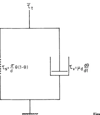
(1982) and Arai et al (1977). They assumed that with the increase in deformation, the restoring elastic stresses due to interfacial tension first increase, pass through a maximum and then decrease. The depicted role of interfacial tension is in the right direction as Rallison (1984) has observed in the context of drop break-up irr shear flows. As the drop approaches the break-up condition, interfacial tension actually aids the fragmentation process. Lagisetty et al (1986) assumed that the force due to interfacial tension reaches zero when the dimensionless deformation of the drop 0 becomes unity. They also assumed that the drop break-up process should be completed within the lifetime of the eddy. Thus, for breakage to occur, the value of 0 should reach unity within the lifetime of the eddy. Their model has been schematically shown in figure 2. The basic equations for their model are:
~'t = Zs + Tv, r, = (tr/d)O, (! - 0,),
= 0,
r,, = z o + K (dO,,/dt)".
0~< 1 0,/>1
(7)
Equation (9) is the general constitutive equation yielding Newtonian, power law and Bingham plastic fluids as special cases. The average turbulent stress in a stirred vessel across a length scale of d is proportional to pcu2(d) and can be expressed as
Z t = Cpc N 2 D */3 d 2/3. (1 O)
As the Voigt model's elements act in parallel,
0 , , = 0 , = 0 . (ll)
Substituting (8), (9), (10) and (1 l) into (7), we obtain
Cpc N 2 D,/3 d2/3 _ Zo = (t~/d) 0( 1 - O) + K (dO/dt) n. (12) Equation (1 l) may be expressed in dimensionless .form as:
C W e ( d / D ) s/3 - (0 - 0 2 ) - (z o d/a) = (d0/dr/) n, (13) (8) (9)
Breakage and coalescence of drops
I
79
dO
Figure 2. A Voigt element.
where r/is the nondimensional time given by t/(Kd/a) w". The initial condition for this equation is give~l by:
0 = 1 , at q = 0 . (14)
Equation (I 4) is solved to find q at 0 = 1. If q at 0 = 1 is more than the nondimensional lifetime of the eddy, breakage would not occur. Thus, for breakage to occur, the following condition must be satisfied:
r/(0 = 1) ~< T/(Kd/tr) 1/". (15)
The maximum diameter of the stable drop is that for which the following equality holds:
r/(0 = 1)= T/(Kdmax/tr) l/~. (16)
The dma x c a n therefore be determined by solving (13), (14) and (16) provided an expression is available for T. Using the turnover time of the eddy as the lifetime of the eddy:
= (1/N)(d/D) 2/3. (17)
Lagisetty et al (1986) have given solutions for various values of n, including the value of unity. They found that the value of C works out to be equal to 8. Their model gives (6) as a limit as K ~ 0 and, with C = 8, the proportionality constant equals 0.125, a value close to that reported by Sprow (1967). The solution for Newtonian fluids is given by
(Re/We)(dmax/D)- t,3 = [1/(4;( - 1) ~ ] t a n - l [!/(4;( - 1)~], (18)
103dmax
/
o 300 rprn /
m
z~ z, O0 / . I
1.5 / I
o 500 /
t r : 0 . 0 2 N/m / /
D : 0.0635 m - - / / / /
o
0 I I t t ~ I i ~ l ~ , ~ J t , , l l
I
0.01 0.1 1.0 Pa.s
Pd
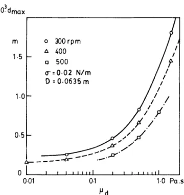
Figure 3. Verification of the model of Lagisetty et al (1986) for the effect of dispersed phase viscosity (.ud) on dm~x. The lines correspond to the theory (18) and are compared with the experimental results of Arai et al (1977).
where Z is equal to 8 We (dmax/D) 5/3. Figure 3 shows a comparison between theoretical predictions and experimental observations for the effect of dispersed phase viscosity on d,,~x. It can be seen that, when interfacial tensionis of the order of 0"02 N/m, d~x is hardly affected by the dispersed phase viscosity till it exceeds about 0-1 Pa.s. They have tested the model using Newtonian, power law and Bingham plastic dispersed phases and report the agreement between the predicted and experimentally obtained values to be good. Some recent measurements on very viscous liquids however seem to indicate that Lagisetty's model overpredicts the value of dm.x under these extreme conditions.
The basic framework of the model has been tested for a number of situations where either surfactants (or drag reducing agents) were added to the continuous phase, or the dispersed phase was a rheologically more complex viscoelastic fluid.
2.2c Breakaye in presence of surfactants: Koshy et al (1988a) have investigated the breakage of dispersed phases when a surfactant is added to the continuous phase.
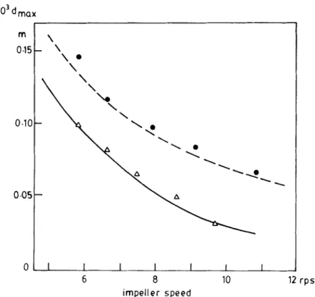
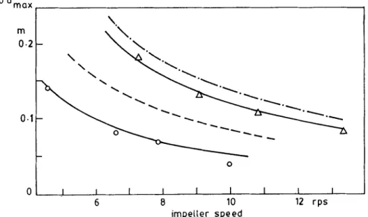
Addition of surfactant could be expected to reduce the drop diameter by reducing the interfacial tension of the system. Two systems with identical interfacial tensions, one with surfactant and the other without it, were studied. The water-octanol system had an interracial tension of 0-0083 N/m and did not have a surfactant. Teepol was added to a water-styrene system to bring its interfaciai tension from 0-034 N/m to 0.0083 N/m. The viscosities of both the dispersed phases were too low to affect dma x and in any case were nearly equal. The values of dmax have been plotted as a function of revolutions per second (rps) for both the systems in figure 4. It is interesting to note that the two systems yield different results and, surprisingly, while (6) explains
B r e a k a g e and coalescence o f drops 81 103 dmax
m t ,
0.15
\Nx,, e
I \ ^ ~ ~ •
0-05 _ \ A ~ ~ . ~ e
0 I I I I I I I
6 8 10 12 rps
impeller speed
Figure 4. Breakage in presence ofsurfactants. The experimental values for the water-octanol system (0) are in good agreement with (6) ( ... ). The best fit line ( - - - ) through the experimental data (A) for a surfactant solution-styrene system having the same fnterfacial tension (0.0083 N/m) indicate lower d,,~x values in the presence of a surfactant.
the results of the w a t e r - o c t a n o l system, using a value of 0" 125 for the constant, it fails to explain the results of the system containing the surfactant. These results indicate that the surfactant not only acts through reduction of the interfacial tension, but also influences the breakage in some other fashion which has not been considered by any of the earlier models.
A pressure fluctuation across a d r o p diameter most probably causes a depression or elongation which propagates, resulting in d r o p breakage. When surfactants are present at the interface, the pressure fluctuation, apart from causing depression at the surface, also removes the adsorbed surfactant molecules thereby exposing fresh interface. This fresh interface has dynamic interfacial tension, which is higher than the static interfaciai tension. This difference in the two interfacial tensions causes a flow towards the base which adds to the flow already taking place due to pressure fluctuation. The assumed mechanism through which the extra stress is generated has been shown in figure 5. The model of Lagisetty et al (1986) has been modified to account for this extra stress as follows:
Cpc N 2 D 4/3 d 2/3 + (Aa/d) - r o = (a/d)O(l - O) + K (dO~dO", (19) where Aa is the difference between the dynamic and static interfacial tension values.
The modified model has been tested by Koshy et al (1988a). Figure 6 shows two sets of experimental data in the range of surfactant concentrations where the dynamic
(
applied turbulent stress
l
(b) .
high ~ ~ due to (o- d -o-)
Figure 5. Mechanism through which a surfactant influences drop breakage. (a) Drop before interation with eddy; (b) formation of the depression.
and equilibrium interfacial tensions differ. F o r both sets of data presented, the system is water,styrene. Different concentrations of Teepol have been used for the two sets.
In one of the sets, the interfacial tension has been reduced to 0.011 N/m while the Aa is 0.0014 N/m. The points are experimental whereas the solid and dotted lines correspond to (19) and to Lagisetty et al's (1986) model respectively. It is evident that the model represented by (19) is able to predict the results correctly while the other overpredicts the dm,, values significantly. Similar conclusions can be drawn from the other set, the interfacial tension and Air for which are 0-0253 and 0-0011 N / m respectively.
lO]dmax
o • 2 \
"~.
\
\
- ~ ~ " ~ ' ~ . ~
0
0 .I I I I I I I I I
6 B 10 12 rps
impeller s p e e d
Figure 6. Effect of surfactant on dma ~ when the dynamic and static interfacial tensions are different. The system is styrene-water and the suffactant used is Teepol. Two different concentrations have been employed-(©): o=0.011N/m; Ao=0"0014N/m and (A):
o = 0-0253 N/m; Aa =0.0011 N/m. The dashed lines represent (18) while the solid lines correspond to the model of Koshy et al 1988a, (19).
Breakage and coalescence of drops 103 d mQx
83
m
0-2
0-1
0 I I I I I I I I
~, 6 8 10 rps
impeller speed
Figure 7. Effect of high concentrations ofsurfactant on din,,. A: pure styrene-water system, a = 0-034 N/m; O: water-Teepol-styrene system, tr -- 0.0032 N/m. The solid lines correspond to the model of Koshy et a11988a, (19).
As the concentration of the surfactant is raised from zero, the Aa first increases and then decreases, eventually becoming zero. Figure 7 shows the results for zero and high concentrations of the surfactant (corresponding to Aa = 0). It is interesting that the experimental results are explained by the model of Lagisetty et al (1986) which is a special case of the model represented by (19). When a very viscous dispersed phase is used, the effect of surfactant is found to be insignificant, as the breakage is controlled mainly by the viscous stresses, with minor changes in interracial tension making negligible contribution.
2.2d Mildly viscoelastic dispersed phases: Koshy et al (1988b) conducted experiments on breakage of viscoelastic fluids by using aqueous solutions of polyacrylamide (Separan AP-30) as the dispersed phase. Two solutions having concentrations of 0"25 and 0"5~o were employed. The drop sizes were much larger than those predicted by the model of Lagisetty et al (1986) for purely viscous drops. This model was therefore modified by Koshy et al (1988b). The modification was mainly concerned with the manner in which a viscoelastic drop deforms. It was assumed that the interaction between an eddy and the drop begins sharply. Under these conditions, the polymer acts as a glass and supports the applied stress without significant deformation. As time progresses, the stress borne by the polymer decreases due to the relaxation of the polymer molecules. The deformation therefore proceeds in this manner with the stress borne by the polymer decreasing continuously. The relaxation of the stress borne by the polymer was assumed to follow the expression:
ru = z, e-'/~, (20)
where 2 is the relaxation time of the polymer. With this modification the equation
103 d mo, x m 2-5
2 (
1.0
05
I I I I I I
6 8 10 12 rps
impeller speed
F i g u r e 8. Verification of the model of Koshy et al (1988b) for viscoelastic liquids. System:
heptane and carbon tetrachloride (specific gravity 1'06)-0.5% aqueous solution of polyacry- lamide, inteffacial tension ---0-057 N/m. A experimental points. - - (21); . . . . (18).
for viscoelastic dispersed phases becomes:
CpeN2 D4/3 d 2/3 + T O = ( t r / d ) O ( I - O) + (CpcN2 D4/3 d2/a)e -t/a +
+ g (dO~dO".
(21)
The d,,ax can be found as before by integrating the above equation with the initial and breakage conditions described earlier. The verification of the model has been shown in figure 8, where dm,x is plotted as a function of rps for 0-5% polyacrylamide solution as the dispersed phase. The points are experimental whereas the solid line is based on the model. The predictions made by the model of Lagisetty et al (1986) are shown as the dotted line, and fall significantly below the observed values of dma x.
The above model has been found to successfully predict the dma~ values only when the dispersed phase is mildly viscoelastic (having time constants of the order of 0.1 s or less). For highly viscoelastic dispersed phases, no drop breakage was observed experimentally. Instead, the dispersed phase was found to be present in the form of big blobs which elongated into thread-like structures when they passed through the impeller zone. The model was unable to predict such behaviour.
Breakage and coalescence o f drops 85 2.2e Breakage in presence o f drag-reducing agents: A number of investigators (Mashelkar et al 1975; Quraishi et al 1976; Hoecker et al 1980) have shown that the addition of small quantities of drag-reducing agents (ORA) to a stirred vessel results in torque suppression, indicating that the turbulent energy pattern gets altered. Thus, the drops formed in such a situation, should be larger than those obtained without the addition of DRA. Walstra (1974) measured average drop size of paraffin oil in a turbomixer by adding polyvinyl alcohol (PvA) to the continuous water phase and found that with increase in PVA concentration, the drop size first decreased and then increased. However when a surfactant was also added, the average drop size increased with increase in PVA concentration. Koshy et al (1989) measured dmax values for a number of systems and found that the addition of even 25 ppm of polyacrylamide to the continuous aqueous phase resulted in an increase in dmax values. They did not use any surfactant in the continuous phase in their experiments. They were able to predict the increase quantitatively by considering that the DRA change the energy budget of the eddies thereby causing a change in the inertial stress. In the elongating eddies, the DRA molecules elongate and store a part of the eddy energy as potential energy. On drop-eddy interaction, the molecules relax releasing a part of the stored energy. The energy available for breakage can be obtained by subtracting the stored energy at any time from the energy of the eddy without drag-reducing agents. Thus
rt = C [pcuZ(d) - (ep~ - ep,)]. (22)
The energy stored by a polymer molecule was evaluated by the finitely extendable elastic dumbbell (FENE) model. The molecule extends because of the difference in velocity across the molecule, but this extension is retarded because of the elastic spring. Finally, the extended molecule reaches an equilibrium size corresponding to the strain rate existing in the eddy. The energy of an extended molecule is:
E~(Ro, d) = f ( H R g I 2 ) I n [1 + ((/HT")]. (23) This equation has to be modified by multiplying the right hand side with d/l T if the eddy size is smaller than the Taylor microscale, IT.
As there will be a molecular weight distribution of the polymer molecules, the overall energy accumulated in all the polymer molecules present per unit volume works out to be:
ep~ = (3/2)(f/n)(pcR o T/mo)w g(p)ln [1 + (4rt22o/67')dp. (24) The above expression also has to be multiplied by d/l~ if the eddy size is smaller than the Taylor microscale, IT. For evaluating the energy released back by the polymer molecules to the eddy, they used the expression:
Ep(l - e r~"). (25)
Taking the molecular weight distribution into account, ep, was found to be:
ew = (3/2)(f/n)(p~R o T/mo)w 0(p)(1 - e-f/~-°)ln [1 + (4n22o/6T)] dp.
(26)
10 3 dmo x
0.1 \ x \
\ A \ 0 . 1 -
0.i --
0 ' 2 -
0 4
", A
~ A
Figure 9.
of polyacrylamide, interracial tension 0-036 N/m. A experimental points; - - Koshy et al (1989), (28).
I I I I I
6 8 lOrps
impeller speed
Effect of a drag reducing agent on d,..x. System: toluene-50 ppm aqueous solution
model of
Substitution of expressions for ep, and e~s in (22) yields:
z, = 8pcu2(d) - 12(f/n)(pcRg T/mo)w g(p)(e-77>°)ln [1 + (4rc2 2o/67")] dp.
(27) The rest of the analysis of Koshy et al (1989) follows the same lines as that of Lagisetty et al (1986). The final expression for dm~ is:
where
( R e / W e ) ( d m ~ j D ) - 1/3 = (4/0t½) t a n - 1 (1/0t½), 0t = 32[We - (z,dm~Jtr) ](dm~z/D) 5/3 - 1,
(28)
and % is the last term of (27). Figure 9 presents a typical comparison between the predicted and experimental values of dm,x as a function of rps for a water-toluene (dispersed) system, when 50ppm of polyacrylamide were added to the continuous (water) phase. It is possible to explain the results obtained for other systems also including the ones containing surfactants, when ORA are added to the continuous phase.
2.2f Variation o f dma x with dispersed phase volume fraction: The turbulence in the stirred vessel is dampened as the volume fraction of the dispersed phase (hold-up) increases. Though there is no theory available to predict the dampening quantitatively,
Breakaqe and coalescence of drops 87 empirical expressions have been proposed to calculate the effect. Typical of such correlations is the following proposed by Laats & Frishman (1974):
[u: (d) ]~, ~ ,~ = (1 + 4~b) - 2 [u 2 (d)-14, = o- (29) Lagisetty et al (1986) have shown that by modifying the turbulent stress in accordance with the above empirical expression, the effect of the hold-up of the dispersed phase on the values of dm~ ~ can be predicted up to a hold-up value of about 0.3.
2.2g Some outstandiny problems: It is seen that our understanding of drop breakage in turbulent stirred dispersions is still at a rudimentary stage. First generation models, which bypass the flow field and simplify the three-dimensional problem to a unidimensional one are however available. These models, though gross, can predict the dma x values for lean dispersions containing viscous drops, though they fail when the dispersed phase is highly viscoelastic or its viscosity is extremely high.
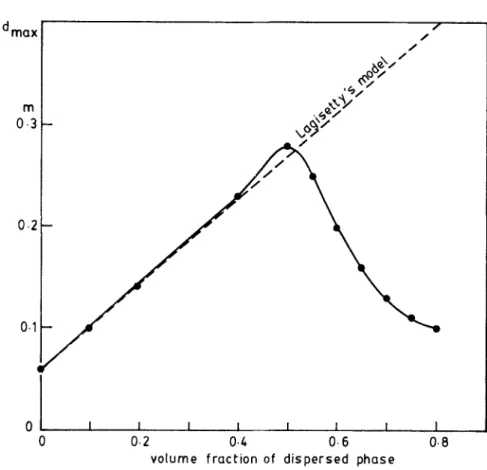
In slightly concentrated dispersions, the turbulence gets suppressed and empirical modifications have to be resorted to for the prediction of dmax. Even these work only up to a dispersed phase hold-up (~b) of about 0.3. Beyond this dispersed phase hold-up, highly unexpected results are obtained. With increased hold-up, the turbulence intensity decreases. Thus the d,~a~ value is expected to rise as ~b is increased. This however happens only up to a ~b of around 0.3, as is seen from figure 10, which presents
dma x a s a function of ~b for the water-toluene system. A surfactant was added to the continuous phase to suppress coalescence, thus making the process predominantly breakage controlled. It is seen from the figure that beyond a value of q~ of around 0.3, the dma ~ values decrease instead of increasing. These results lead one to speculate that under such conditions, the d,,a~ is not decided by the turbulent breakage mechanism as this would yield an increase in d,,~. Instead d,,~x is now decided by other mechanisms. One possibility is that the drops break in the extensional flow generated at the impeller by the liquid approaching the impeller in the middle and accelerating outwards. The second possibility is the drop breakage in the boundary layer existing at the impeller. Here shear breakage would be predominant. Though the magnitudes of elongational rates and shear rates are different, both mechanisms yield a lowering of drop size with ~b which is in qualitative agreement with observed trends. Thus it is likely that the experimentally observed d=~x is the minimum of the dm~ values generated by these different (viz. turbulent, elongational flow and shear flow) mechanisms. Further conceptual complications arise in the case of concentrated suspensions. For instance, in such media, should suspension viscosity be used for characterizing the continuous phase? Further, what modifications are needed in the theory if the viscosity of the dispersion is such that the tip Reynolds number is reduced below 104? A reduction by a factor of ten, which would imply that flow is still turbulent, is perhaps the case in most emulsifiers.
The models discussed above have accounted for the breakage occurring in the impeller zone since that is relevant for calculation of dmax. However, the breakage that occurs in other areas of the stirred vessel, where shear forces may also be simultaneously important, would also be needed for calculating the drop-size distributions.
Apart from these lacunae, there remain several other conceptual questions. The above models do not really account for the eddy-drop interaction in a mechanistic way. Further, they adopt an arbitrary breakage condition. Thus, does the drop break
lOZdma x
m
0-3
f f J
- ~
0.2
0.1
0 I I I I I I I I
0 0.2 0.4 0.6 0.8
volume fraction of d i s p e r s e d phase
Figure 10. Variation of d=. x with dispersed phase hold-up. The dispersed phase is toluene.
The continuous phase (water) contains 0.3% sodium lauryl sulphate to suppress coalescence.
The solid line through the experimental points diverges from the model predictions of Lagisetty et al (1986) beyond a hold-up of 0-3.
by surface tension driven instability or by the end-pinching mechanism observed in laminar flows or by an entirely different process? The black box approach towards d r o p - e d d y interaction is also silent on the details of the nature of the flow that occurs inside the drop. For instance, is it elongational or shear in nature? An answer to this question may hold the key to explaining the failure to disperse highly viscoelastic dispersed phases.
Finally it would be interesting to see if the model of Lagisetty et al (1986) can be used in other equipment, such as pulsed columns, nozzles etc. by making appropriate substitution for e, the power dissipation per unit mass.
Thus even for dm~ evaluation, there is need for more robust models which could account for d r o p - e d d y interaction in a more acceptable fashion, take detailed flow field into account and incorporate a more realistic breakage condition.
2,3 Breakaoefrequency
The evaluation of dm=, though useful for calculating the average drop diameter existing in the vessel, cannot yield the drop.size distribution. To obtain this, it is necessary to solve the population balance equations, which in turn require expressions for breakage frequency, coalescence frequency and the size distribution of the daughter droplets formed through the breakage of a larger drop.
Breaka¢le and coalescence of drops 89 Breakage frequency [F(v)] can be physically interpreted as the fraction of drops of a given size v that break in unit time when they are kept in a turbulent flow field.
In view of the time invariance of the statistical properties of the turbulence, it is also a measure of the transitional breakage probability of one such drop i.e. F(v)dt is the probability of a drop of size v undergoing breakage in a small time interval dt. Its average value for a given drop size may, therefore, be computed as the reciprocal of the expected survival time of such a drop in the turbulent environment under consideration. A reliable model for this is necessary to enable us to solve the population balance equation and obtain the drop-size distribution. Models are available in the literature which try to predict breakage frequency for inviscid dispersed phases, which undergo instantaneous breakage. There is no reported model which attempts to predict breakage frequency for dispersed phases which have finite viscosities or which display more complex rheological behaviour.
2.3a Models for breakage frequency: Early models of breakage frequency have been either ad hoc or have drawn upon analogies to rate expressions characteristic of chemical reactions. Thus Valentas & Amundson (1968) have assumed the breakage frequency (regarded as a function of the drop diameter, d, in this section) to be proportional to the droplet surface area:
F(d) = C 1 d 2. (30)
Ross & Curl (1973) saw a similarity between drop breakage and chemical decomposition. They assumed a drop to form an 'activated complex' due to imparted kinetic energy, which then broke just like a chemical reaction. Thus:
K "
normal drops,-~-~'activated drops' ~ breakage products,
where the normal drops are in equilibrium with the activated drops and K" is the rate constant for the decomposition or the break-up process. The breakage frequency is thus simply
F(d) = K*K", (31)
where K* is the equilibrium constant for the normal-activated drop exchange. From similarity to molecular decomposition,
K* = e x p ( - activation energy/kinetic energy). (32) The kinetic energy is assumed to come from all eddies smaller than the drop since larger eddies would be expected to convect the drop without breaking it. The activation energy is taken to be proportional to ~rd 2 where cr is the interfacial tension. Their final expression is:
F(d) = C 1 NDZ"3d - 2/3 exp [ - C 2 tx/(peN2D4/3dS/a)]. (33) The two unknown parameters C1 and C 2 are determined from the experimental data to obtain the best fit.
Coulaloglou & Tavlarides (1977) define the breakage frequency on more physical grounds as:
FId) = (1/breakage timel x number fraction of drops of size d
breaking in that time. (34)
They assumed that the fraction of drops breaking is proportional to the fraction of drops of size d which have a total kinetic energy greater than a minimum value necessary to overcome the surface energy holding the drop intact. This minimum surface energy was taken as
E c oc trd 2. (35)
Using the two-dimensional normal distribution for the velocity fluctuations of the eddies, they derived an expression for the fraction of eddies with kinetic energies exceeding Ec:
framon of eddies with E > Ec --- exp [ - (EriE,)]. (36) Here Et is the kinetic turbulent energy of an eddy of size d and is related to the energy dissipation per unit mass by
E t oc pc~,2/3d 11/3. (37)
They estimate the time available for breakage to be
tb = d2/3e - 1/3, (38)
from consideration of the relative motion of two lumps of fluid in a turbulent flow field as described by Batchelor (1953). In terms of the operating parameters of the stirred vessel, their final expression is:
F(d) = K 1 d- 2/3 N D2/3 exp [ - K 2 tr/(pcD 4/3 N 2 d 5/3)], (39) where K~ and K2 are parameters to be determined from experimental data. As is evident, the dispersed phase viscosity has been ignored in the development of the breakage frequency expression. In addition, the idea of time required for the centres of mass of the would-be daughter droplets to separate may have little to do with the breakage phenomenon because during fragmentation itself the parent drop is quite deformed and would give rise to already separated daughter droplets.
Narsimhan et al (1979) view the droplet as a one-dimensional simple harmonic oscillator, oscillating about its spherical equilibrium shape. Oscillations are induced by the arrival of eddies of different energies at the surface of the droplet. They argue that the increase in the surface energy required for fragmentation is minimum if binary equal breakage occurs and has the value
(21/3 __ l)o'n 1/362/3/~2/3, (40)
for a drop of volume o. The arrival of eddies at the surface of a drop is assumed to be a Poisson process with a parameter ). independent of the droplet diameter. The arriving eddy has a kinetic energy per unit mass of ½ u 2 where u is an associated characteristic velocity. To be able to break the drop, therefore, one must have
½u'/> (21/3 - 1)trltl/a62/aoz/a/(pcu). (41)
Assuming that the joint probability distribution of 2 point-velocities in an agitated vessel is normal with a variance
tr 2 = 2 ( e d ) 2/3, (42)
Breakage and coalescence o f drops 91 they arrive at the following expression for the breakage frequency
F(d) = 2 erfc [x/a(n/6)- 1/6d- s/6/(2~- 1/3)], (43) where
a = 2(2 l/3 -- l)rtl/362/3(a/pc). (44)
Das (1984) points out that even though the drop gets to interact with an eddy of sufficiently high energy, the breakage itself need not be instantaneous. Furthermore, there is a finite probability of the nascent daughter droplets recombining which has not been accounted for in the above model. He has modified this model by considering the possibility of recombination of the daughter droplet s also.
None of the foregoing models addresses the situation wherein the dispersed phase has a finite, non-zero viscosity. As the breakage of drops of size dmax is not possible, the size distributions generated by these models contain drops predominantly in the region of dmax. Experimentally obtained distributions however contain drops much smaller than dmax. Furthermore, they yield no information about the daughter droplet distribution fl(v, v') and subsequent use of these breakage models in the population balance equation has to be coupled with independent assumptions about fl(v, v'). In the absence of a phenomenological model, it has been the practice to assume expressions for fl(v,v') that render the population balance equations analytically tractable. Thus, uniform breakage [B(v, v') = I/v'], equal breakage [B(v, v') = 6(v - v'/2)]
and 'normal' breakage {fl(v, v') = [a(2n) l / z ] - 1 exp [ - (v - v'/2)2/2tr 2] } have been reported in the literature (Narsimhan et. al 1979; Shiloh et al 1973; Coulaloglou &
Tavlarides 1977).
Nambiar and others (D K R Nambiar, T R Das, R Kumar & K S Gandhi, unpublished) have recently developed a model which not only predicts the breakage frequency IF(v)], but also fl(v,.v'). These authors consider the possibility of unequal breakage of drops larger than d.~ax. They find that once the drop's diameter has a value of dmax or lower, it cannot be further broken. However larger drops can undergo unequal breakage yielding very small drops which are observed in actual experiments.
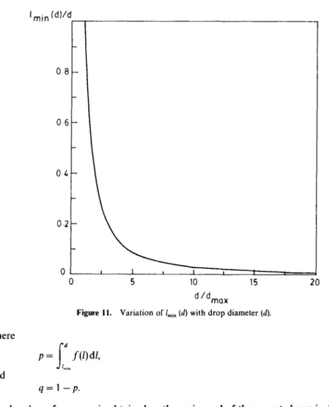
It is found that for a drop of given size, there is a range of eddy sizes whose interaction with the drop can result in its breakage. The size range of eddies (lml . ~< I ~< d) capable of breaking a drop of size d has been obtained through a slightly modified version of the model of Lagisetty et al (1986). The variation of lmi.(d) with the drop diameter, d, is shown in figure 11. It is seen that for d . . . . the ratio of Im~.(d)/d is unity, indicating that smaller eddies cannot break the drop. To obtain the breakage frequency, the drop is permitted to interact sequentially with eddies of various sizes existing in the vessel. If the drop interacts with an eddy much larger in size than itself, it will be simply convected and no breakage will result. Similarly if an eddy of size lesser than I.,i.(d) interacts with it, the drop will get slightly deformed but will not break. It is only when an eddy having size greater than lm~.(d) and less than d interacts with it that breakage will occur. The eddy-size distribution evaluated on the basis of the energy cascade hypothesis is
f ( l ) = 2(Dlr,)2/[(D 2 - l~)/3]. (45)
With this eddy size distribution, the expression for the expected survival time of a drop, tex, works out to be:
fo fo
tex = (q/p) Z-l'(l).f[ll I¢(lm~ . , d)] dl + th(l, d ) f [ l l le(Im~ ., d)] dl, (46)
h
Imi n ( d } / d
08
06
04
0.2
I i I , I i I
0 5 10 15 20
d/dma x
Figure ! 1. Variation of lmi n (d) with drop diameter (d).
where
and p =
f/
d f ( l ) d / , (47)mln
q = I - p. (48)
The breakage frequency is obtained as the reciprocal of the expected survival time,
F(v) = 1/tex. (49)
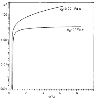
A typical comparison of the variation of the breakage frequency with drop size with the variation predicted through (49) is shown in figure 12. The effect of raising the dispersed phase viscosity hundred-fold has also been indicated in the figure. The breakage frequency tends to be lower in this case. Figure 13 shows the results of a numerical solution of the population balance equation incorporating the above expression, (49), for F(v) and neglecting coalescence. The initial population in this case consists of uniformly sized particles of size 10 dma x. The cumulative volume fraction evolves until no drops of size exceeding dmax survive in the system. The solid line in figure 13 shows the steady state size distribution obtained experimentally by Narsimhan et a/(1980) using an encapsulation technique. It is difficult to describe the initial size distribution in experiments on a batch system to any degree of accuracy and this makes comparison of transient size distributions with numerical solutions difficult. It is reasonable to believe, though, that the steady state size distribution should be independent of the initial conditions.
Breakage and coalescence of drops 93
S_I"
100.
,°° l
0 011
o ooo~ I
0
Pd:O 001 Pa
sr l l l l l l r r l l l r r t l l l l l r l l l l l l l l l l t r t l l l l t l r l l l r
2 4 6 B
103d
Figure 12. Variation of the breakage frequency (F) with drop diameter (d). The effect of increasing the dispersed phase viscosity (#a) is also indicated.
The daughter droplet distribution may be obtained directly from the eddy size distribution using the geometric relation between the daughter droplet volume v' and the size I of the eddy-causing breakage (Papoulis 1984, p. 95).
fl(t", t,) = ½ { f (l[lmi . <~ l <~ d) }/{ i(dv'/dl)[ }.
If the angle ~b is defined by
(50)
cos(O) = 1 -- (2v'/v), (51)
the final expression for fl(v', v) becomes
[3(v', v) = {8(Dlr)2/[prqD 2 - l~)14d] } [sin I(z~/3) - (2~k/3)l/sin ~k]. (52) It is seen from this expression that for binary breakage, equal breakage, which has been hitherto a standard assumption, is more of an exception than the rule.
2.3b Comments on breakage frequency models: Breakage frequency is not measured directly but is extracted from the evolution of the drop size distribution with time in a stirred vessel, under conditions where breakage is predominant. This is normally achieved through using low dispersed phase hold-up. The method of extraction of breakage frequency information from the evolving drop size distribution has been described by Narsimhan et al (1984). The existing models of breakage frequency have not been rigorously tested even when the dispersed phase viscosity is low. For dispersed phases of high viscosity, the only model is that of Nambiar and others (D K R Nambiar, T R Das, R Kumar & K S Gandhi, unpublished) and it has not been tested against any experimental data, as such data are not available. Similar is the
F(dA) 1.0
0 8
0.6
N- 5 rps or_ 0 037 N/m D - 0 0 7 6 2 m dma x -315 xl0"4m
f / / f l It
I t = = / II
I 6°2 " "" rl
l/ I I I
II I II
0 ~ i II I I I II
ii ! II
/1 / / II
/1 / II
0.2 / / 15s / " II
v ,, S.O~--" "" I
0 , , ' ' ' l l r I I I r l r l l l I " I I I I l U I ' I I I 1 1 1 1 1 ! I I I I I l ' I I I I 1 , 1 , 1 t
0.I I 0 I0 0
d i d m a x
Figure 13. Numerical solution of the population balance equation showing the evolution of the cumulative volume fraction F(d, t) with time. F(d, t) is the contribution at time t to the dispersed phase volume fraction from drops of diameter not exceeding d. The initial dispersion is monodisperse particles of size 10 d,~=x. The solid line shows the steady state size distribution obtained experimentally by Narsimhan et al (1980) for the same parameter values.
situation for dispersed phases displaying more complex rheological behaviour. Thus there is need for experimental information so that existing models can be tested and new models developed if necessary.
When the dispersed phase hold-up becomes high, other mechanisms of breakage involving flow at the impeller become important. For such breakage mechanisms, there are no models available for breakage frequency and entirely new models are required to be developed.
Expressions for [3(v, v') are normally assumed. Equation (52) is the only expression based on a mechanistic model. At present, it is not possible to recommend any particular expression for ~(v, v') as the experimental measurement of B(v, v') has not been possible.
2.4 Coalescence frequency
The other most important term required for the solution of the population balance equation is the coalescence frequency. Its prediction involves an analysis of the relative motion between drops. For two drops to coalesce, they must first come very close to each other and then the intervening liquid film between them must drain to such a thickness that it becomes unstable and ruptures. Therefore the problem is normally approached through a two-step procedure. Collision frequency is first computed from an estimation of the diffusion coefficients of different droplets in an isotropic turbulent field. This is then multiplied by coalescence efficiency to account for the complex hydrodynamic interactions that are ignored in the first step.
Breakaoe and coalescence of drops 95 2.4a Models for collision frequency: Smoluchowski (1917), and later Harper (1936) have considered the problem of determining the collision frequency of spherical particles subject to thermal agitation. Two particles of radii r 1 and r2 may be said to be in collision when the distance between their centres is s = rl + r2. According to the theory, if D~ and D2 be the Brownian diffusivities of the two kinds of particles in a binary mixture wherein their number densities are nl and n2 respectively, the frequency of collisions between them per unit volume of the system is given by
v' = 41tnln2s(Dl + D2). (53)
Howarth (1964) reasoned that the above expression could also be used to predict the frequency of collisions between spherical particles suspended in an isotropic, turbulent field, it only being necessary to account for the enhanced diffusivity that is characteristic, in general, of turbulence. For isotropic turbulence, when the diffusion times are short in relation to the Lagrangian integral time scale, the diffusion coefficient is time dependent and is given by (Taylor 1921)
D t = u2 t, (54)
where u 2 is the mean square Lagragian turbulent velocity fluctuation. The time available for diffusion is of the order of the reciprocal of the collision frequency. Thus Howarth (1964) estimates the frequency of collision as
Vc = (4nnsu 2 )½. (55)
An alternative approach to the problem of inter-particle collisions in a turbulent medium is supplied by the kinetic theory of gases. The droplets under consideration here are larger than the microscale of turbulence. They are not therefore completely entrained by the turbulent eddies. The impact of eddies on them in all directions causes them to move,in a random fashion mimicking the random motion of molecules in an ideal gas. Based on this concept, Coulaloglou & Tavlarides (1977) provide the following expression for the collision frequency between drops of volume v and v':
v(v, v') = (9r~}/2)(v} + v'})[u2(v) + u2(v') ] ½. (56) The above expression is typical of this approach and variations, differing from the above only marginally, have been proposed by several other workers (Rietema 1964;
Kuboi et al 1974; Abrahamson 1975).
Both the above approaches to collision frequency are extensions of the existing theories to domains outside the regime of their strict validity. The diffusing elements in Taylor's theory are indistinguishable from the fluid and extension of this concept to macroparticles that alter the flow field around them is open to argument. The kinetic theory models, on the other hand, are intuitive generalizations and their validity comes into serious question when extended to turbulence in a stirred vessel.
However, in the absence of more realistic models, one of the models described above is normally employed.
2.4b Models for coalescence efficiency: The models for the collision frequency clearly view the droplets as hard spheres consequently ignoring th finer details of droplet deformation, the thinning of the intervening film and its rupture at a critical value of thickness. These details are considered in defining the coalescence efficiency which estimates the proportion of collisions that actually result in coalescence.
Howarth (1964) has developed an expression for the coalescence efficiency by deeming coalescence between two drops to occur if the relative velocity along the line of their centres exceeds a critical value. By assuming that the three-dimensional Maxwell's equation describes the drop turbulent velocity fluctuations, he obtained the coalescence efficiency as the fraction of drops which have kinetic energy exceeding the critical value W*. Thus the coalescence efficiency between drops of volume v and v' is given by
q = exp ( - 3 W * / 4 u z), (57)
where u 2 is the mean square turbulent velocity fluctuation.
Coulaloglou & Tavlarides (1977) have assumed the following form for the coalescence efficiency:
r/= e x p ( - to~t). (58)
Here ~ and Fare the mean coalescence time and the mean contact time respectively.
The mean contact time is estimated by viewing the coalescing droplet pair as being entrained in an eddy of length scale d, where d is the sum of the diameters of the coalescing droplets. The contact time is then the mean lifetime of such an eddy,
-t= e 1/3 d 2/3. (59)
The coalescence time ~ is the time taken for the intervening liquid film to drain from an initial thickness h o to critical film thickness h~ under the action of a net squeezing force F effected by the turbulent environment. For drainage between deformed spheres, Chappelear (1961) gives the drainage time as
t - - t o = (3/xcF/16~tr 2) [ ( 1 / h 2) - (1/ho~)] [dd'/(d + d ' ) ] 2. (60) The force is estimated as
F = p~u 2 [dd'/(d + d')] 2, (6l)
where
- - 2 t 2
u 2 = ex(d + d )~. (62)
Their final expression for the coalescence efficiency is
r/= e x p { ( - kp~pe/a2)[dd'/(d + d')] 2 }, (63) where k is a parameter.
Das (1984) and Das et al (1987) recognize the stochastic nature of the drainage process. The drainage equation is that for the thinning of a film of viscous liquid trapped between two rigid, unequal spheres under the action of a squeezing force F directed along their line of centres. Unlike earlier deterministic models, however, the drainage is treated as a stochastic process. If the autocorrelation time of the force fluctuations is far smaller than the characteristic time of drainage, the fluctuations may be viewed as white noise (Das et a11987) superimposed on a constant mean value:
F = ff - 6x/T(,. (64)
Here ~, is a Gaussian white noise process and F and 6 are, respectively, the mean
Breakage and coalescence of drops 97 and standard deviation of the force F. The parameter T is the autocorrelation time of the force fluctuations. With this assumption, the drainage equation
dh/dt = (2hF/3nl~c)[ (1/d) + (1/d')] 2 (65)
becomes a stochastic differential equation and is seen to be completely equivalent to the random, one-dimensional Brownian motion of a hypothetical particle in a bounded interval on the coordinate axis of the variable x = ln(h/hc) with a steady drift towards the origin. The F o k k e r - P l a n c k equation describing the evolution of the transitional probability density is
D*(t32 p/~.x 2 ) q- (Op/t~x) --- (6~p/Oz), (66)
where
r = e f t ; ~ = (2/3rcgc)[(1/d) +(l/d')] 2, (67)
D* = ~6T/(2ff /6), (68)
and p = p(x,r]xo,O)= probability that the particle is at location x at time r given that its initial location was Xo.
The initial condition is an assertion of the film thickness at the start of the drainage process:
p(x, 01Xo, 0) = O(x - xo). (69)
The boundary conditions are:
p(0, rlXo, 0) = 0, (70)
D* PP ...
- ~.~c = ( 1
+k,,,)pl
. . . . - ( 7 1 )The first of these corresponds to an absorbing wall at x = 0 which indicates that rupture is immediate and the coalescence process gets terminated whenever h = he.
The second boundary condition assigns to the particle a finite probability of escape from the interval through its right end-point x = Xo. Physically this implies that the collisional state of the droplet pair may be terminated and the droplet pair may be separated at their initial separation h o. If it is further assumed that the collision time is very large in relation to the time scales over which the fate of the particle pair (coalescence or separation) is decided, the efficiency of coalescence is obtained as
r/= probability that the Brownian particle will ever be absorbed at x = 0
• c~p
= fo x O*~x x x=odr. (72)
For coalescence between drops of diameters d and d', the standard deviation of the force fluctuations in the above model has been taken to be
= pcu2(d + d') [dd'fld + d')] 2. (73)
The mean value of the force is assumed to be proportional to 6 with the proportionality constant expected to decrease with increasing intensity of turbulence. The auto- correlation time T has been assigned a constant value of 10 -4.