These variations depend on the physical appearance of a person such as height, weight etc. The size of the kidneys also varies in diseases such as diabetes and cysts. Sometimes the entire portion of the kidney is not observed due to occlusions of other organs.
Evaluation
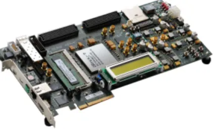
Acquisition System
The third part consists of signal processing techniques to process the received high dynamic range data and finally display the ultrasound image.
B-Mode Image Processing
The envelope of the high dynamic range demodulated signal is detected from the RF data and needs to be compressed to match the dynamic range of the human eye. Scan transformation includes linear interpolation and address transformation between adjacent pixel values to smooth out the effects of coordinate resampling as described to avoid unnecessary artifacts and provide a better user interface.
Ultrasound Backend System Architecture
The actual dynamic range of the received signal is about 80dB or higher depending on the ADC bits of the amplifier. Since the maximum dynamic range of the human eye is in the order of 30 dB [43], the log transform is used to compress the pixel values that have the dynamic range of 80 dB to the desired range [39].
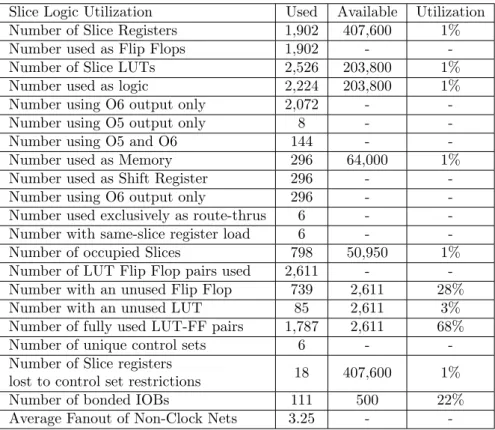
FPGA based Backend System Implementation and Results
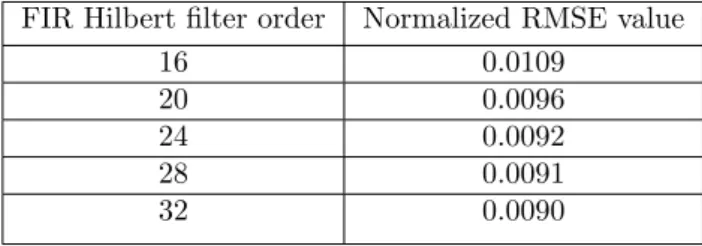
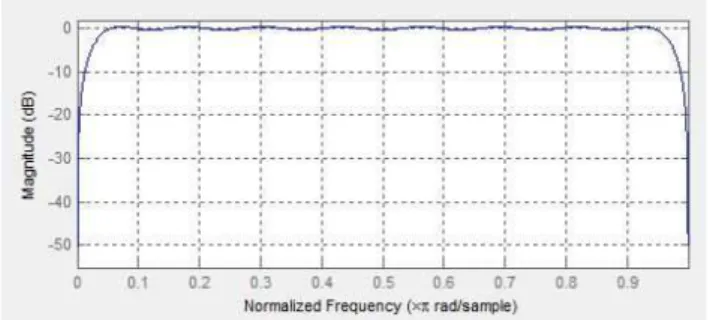
Referring to Table 2.1, 32-tap filter gives the least RMSE (0.0090), and therefore we implemented 32-tap FIR Hilbert filter with the magnitude response shown in Fig. The quadrature components obtained from the Hilbert filter block are passed through the envelope detector to detect the envelope of the RF signal.
Conclusion
For large values of N the echo can be expressed as e(t) =Acos(ω0t)−Bsin(ω0t) (3.2) According to the central limit theorem, A and B are identical Gaussian random variables with zero mean and are given by . For m= 0.5 half Gaussian is obtained, m= 1 we get Rayleigh and for values m > 1 we get Rician distribution.
Envelope Compression in B-Scan Imaging
Logarithmic Compression
Gamma Compression
Wavelet based Compression
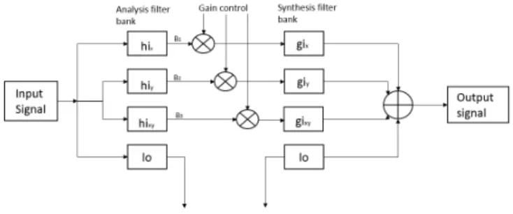
The filter taps of the analysis filter bank are staggered and padded with zeros, the high-pass filterf1 increases from [1,−1] initially to [1,0,−1] and later in the subsequent stages, similarly low-pass filterf0= [1,1 ] is padded with zeros, resulting in 2Dzero padded filters (hix, hiy, hixy, lo) whenf0. The gain control depends on the activity map which varies from point to point, and therefore the gain map is formed depending on the subband image. Single gain mapGag =p(Aag), where p(.) is a non-linear function given by p(Ai) =. 3.19) where γ is a compression factor between 0 and 1, ε is a parameter related to the noise level, δ is the stability level of the gain control set to one tenth of the Aag average.
Results
The compression techniques are assessed based on several visual quality assessment indices, including Multi-scale SSIM index (MSSIM), Structural SIMilarity (SSIM) index, Pixel-based Visual Information Fidelity (VIFP), and Peak Signal-to-noise ratio (PSNR). The SSIM index measures image quality using an initially uncompressed image as a reference with the other images. MS-SIM values are obtained by calculating values of cross-correlation and variance of the image at different scales, obtained by low-pass filtering and sub-sampling, by a factor of 2 in spatial directionsx andy [51].
Mutual information between input and output of the Human Visual System (HVS) channel of the reference image is then compared with HVS. c) Gamma compression (d) Wavelet-based compression Figure 3.3: US image with different compression techniques. It is clear from the table that the gamma compressed image matches well with the original uncompressed image compared to other compression techniques such as log compression and wavelet compression technique.
Conclusion
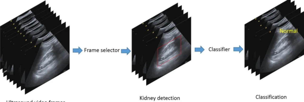
Preliminary CAD is used to classify normal and abnormal kidney images, and not further classify into abnormalities such as cysts, stones, etc. After noise removal, organ features are automatically extracted by our proposed algorithm, from the extracted features, only some are selected by feature selection algorithm, to validate any anomaly in the organ in the classification block. Based on the classification decision, the priority of sending patient data in case of emergency can be changed to high.
In the wavelet domain, the original image coefficients will be of large value, and when noise is added to the original image, the value of the coefficients will be small. The discrete wavelet transform (DWT) of the image is computed at three levels of decomposition and thresholding is applied to these levels.
![Fig. 4.1 shows the FPGA based CAD implementation of the classifier to determine the abnormality of organ [22] in ultrasound images](https://thumb-ap.123doks.com/thumbv2/azpdfnet/10530251.0/28.892.356.563.722.809/shows-fpga-implementation-classifier-determine-abnormality-ultrasound-images.webp)
Feature Extraction
Therefore, coefficients with smaller values indicating the presence of noise are set to zero to eliminate noise. Global threshold is applied according to which values below the threshold are set to zero and the remaining values are set to start from zeros. Inverse Discrete Wavelet Transform (IDWT) is performed on the resulting wavelet coefficients to obtain the noise-laden image.
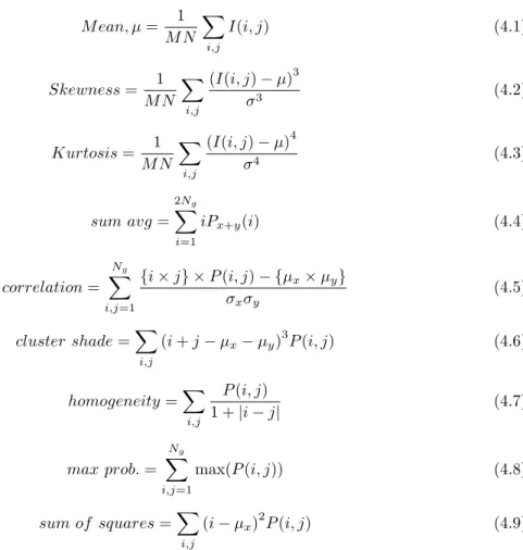
Comparative studies between two kidneys are necessary to obtain adaptive characteristics, such as determining the change in kidney size. There are 22 Haralick features, including contrast, autocorrelation, correlation, cluster shadow, cluster prominence, dissimilarity, maximum likelihood, homogeneity, sum of squares, sum mean, sum variance, sum entropy, difference variance, etc.
Feature Selection
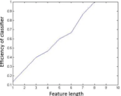
These properties are extracted from the co-occurrence matrix Gof dimensionN g (number of gray levels) as given below, each element P(i;j) gives the probability of occurrence of gray levels in the specified spatial relationship with gray level j. For our application, to determine abnormality in kidney, algorithm completed at third generation (ie atk=3) and finally 12 features (Pk=12) are obtained as an output of GA. Since the efficiency is constant, from parameter length 8, 9 and 10, out of 12 features obtained, only 9 features are selected for further analysis.
The selected features include mean, skewness, kurtosis, cluster shadow, correlation, sum mean, maximum likelihood, homogeneity, sum of squares, longitudinal length of the kidney is considered as the 10th feature. Finally, these 10 optimized features are considered for further classification instead of considering all features.
Classifier
In Table 4.1, the length is a flexible feature and should be trained each time depending on the patient, for example, in the case of diabetics, the kidney size will be more than 12 cm, but this case should be defined as normal. Depending on the patient's condition, the longitudinal length of a normal kidney is considered a threshold. The intervals are then compared to the threshold values and if any feature exceeds the threshold value, the classifier decides that the kidney is abnormal and sends the data to the cloud with a high priority, requesting a doctor for an immediate diagnosis.
If all the functions are within the normal range, data is sent to the cloud, without any priority, doctors can review reports whenever possible. The proposed CAD algorithm is ported on FPGA for validation, true positives and true negatives are calculated on a database of 394 images.
Hardware Complexity Analysis of proposed CAD algorithm
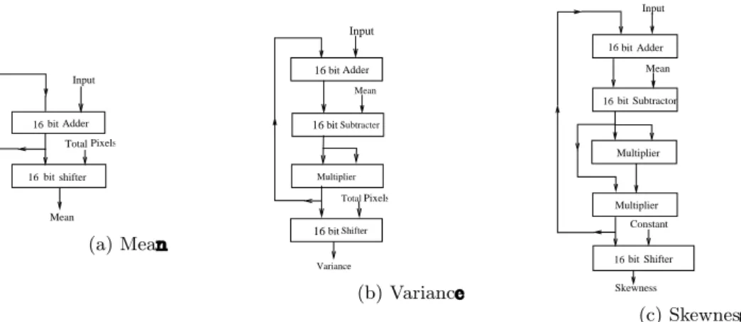
Complexity analysis for feature extraction
To find the product of the constant K6, a multiplier is required, defined as the mutual probability obtained from the GLCM and image index functions, both inputs are given to the multiplier, and a subsequent 16-bit adder is used to sum the values obtained from the multiplier. The resulting result is subtracted from the product of mean x and mean y, which are the averages along the x and y axes using a 16-bit subtracter. It requires two 16-bit adders, one to add the sum of the indices and another to add the mean values along the x and y axes.
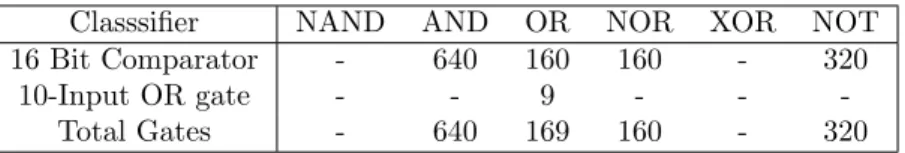
It requires 16-bit comparator to find maximum likelihood and 16-bit adder to the sum of maximum likelihood of each element in the GLCM matrix. It requires 16-bit subtractor to find difference between element index along x-axis and average along x-axis.
Complexity analysis for classifier
The kernel is shifted from the top left of the image by one pixel and the new feature value is calculated. Similarly the kernel is then moved through the entire image until it reaches the right end of the image and all feature values are calculated. The process is repeated until the kernel size reaches the window size.
In an integral image, the sum of all pixels under a rectangle can be evaluated using only the four corner values of the image. Later, the weight of the misclassified examples is increased and the process continues until the required number of features are selected.
Abnormality detection
Feature Extraction
After determining the ROI in the ultrasound image, features are calculated to classify whether the image is normal or abnormal.
SVM Classifier
The features considered when training an SVM classifier are mean, variance, standard deviation, skewness, kurtosis, and entropy. When an ultrasound image of a kidney is given as input, the kidney is detected in the image using a kidney detection algorithm and its features are calculated.
Results
Database
Metrics used for evaluating alogrithm
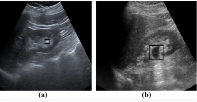
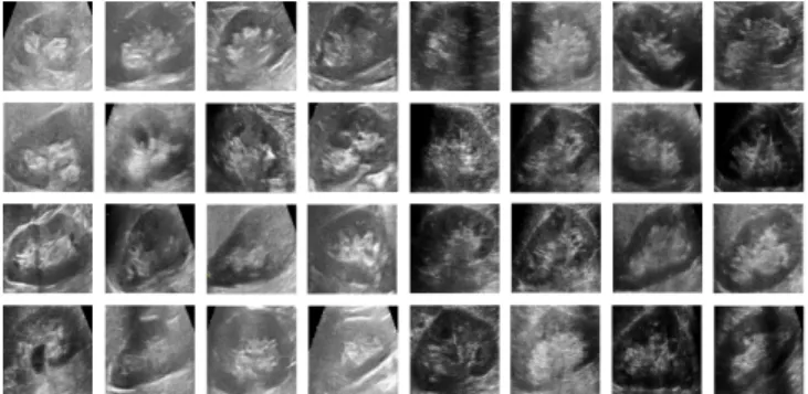
640 kidney images were used for training the Viola Jones algorithm, of which 320 are positive kidney images as shown in Fig. The set of positive data also includes kidneys with abnormalities such as cyst, infection, stone, etc. For the training of the Viola Jones algorithm, we manually marked the kidney images in the presence of the sonographer. The Viola Jones algorithm is initialized with the following parameters: the window magnification at each step is set to 1.1, the minimum initial window size is set to 24×24 pixels.
To detect abnormalities in the image after localization, we used 300 images to train the SVM classifier (with RBF kernel), of which 150 are normal cases and 150 are abnormal cases (consisting of stones, cysts). The performance of the proposed algorithm is tabulated in the confusion matrix as shown in Fig.
Conclusion
Computer Aided Diagnosis for Kidney
A single portable FPGA-based ultrasound imaging system for point-of-care applications.” Ultrasound, Ferroelectrics and Frequency Control, IEEE Transactions on. 24] Jun Xie; Yifeng Jiang; Hung-Tat Tsui, “Kidney segmentation from ultrasound images based on prior textures and shapes,” Medical Imaging, IEEE Transactions on, vol. 37] Mawia Ahmed Hassan and Yasser Mostafa Kadah, “Digital Signal Processing Methodologies for Conventional Digital Medical Ultrasound Imaging Systems,” IEEE Trans American Journal of Biomedical Engineering [online.
Bovik, "Multiscale Structural Similarity for Image Quality Assessment," IEEE Asilomar Conference Signals, Systems and Computers, Nov.