The main objective of the research is to propose a new algorithm for better k forecasting, which can further be used for dry weather streamflow forecasting. Examining the anomaly of the relationship of the recession coefficient k with past flow for California basins and investigating the causes of the anomaly.
Organization of Thesis
Analysis of the recession flow provides important information about the storage characteristics of the basin, as it mainly concerns the subsurface flow. This can be done by identifying the patterns in the recession events and by connecting to the physical properties of the basin using analytical models. Most recession studies suffer from the fact that there is no theory that captures the exact onset of the recession flow.
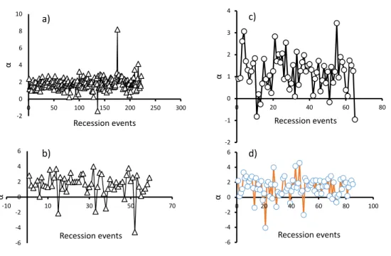
Variability of recession constants (k and α)
Recession flow definition
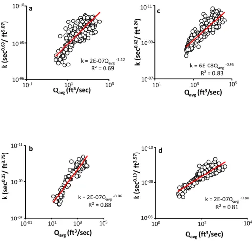
Anomaly of recession coefficient k and past discharge
In our study, by investigating the above behavior, a generalized algorithm is proposed for a better prediction of dry weather flow and consequently (using equations 2.9, 2.10). Our approach only needs past discharge and can be satisfactorily applied to any basin that is free of human interference.
Model Evaluation Statistics
Model Evaluation Statistics (Dimensionless)
It is a standardized measure of prediction error and ranges from 0 to 1, where 0 means no relationship and 1 is a perfect relationship between modeled and observed values. An NSE value of 1 means that the predicted and observed values are exactly the same, and 0 means that the model is as accurate as the average of the observed values.
Model Evaluation Statistics (Error Index)
Gravity corrections
Latitude correction
Free air correction (Free-air gravity anomaly)
Bouguer slab correction
Corrected Bouger gravity for terrain (∆g tb )
Correction due to pressure
Correction for ground water level change
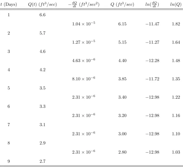
Half of the available data were used for calibration of recession parameters (kN0, λN) and the remaining data were used for validation. Fixing αof the basin as the median of the distribution of α values of individual recession events and back-calculating k.
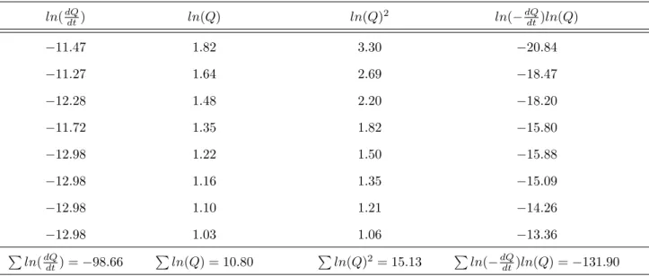
Calculation of recession constants α and k
Calculation of k after fixing α
For the same pool 03368000 and for the first recession period (α of the pool is fixed as the median α of the distribution of all individual recession events and is observed as 1.83).
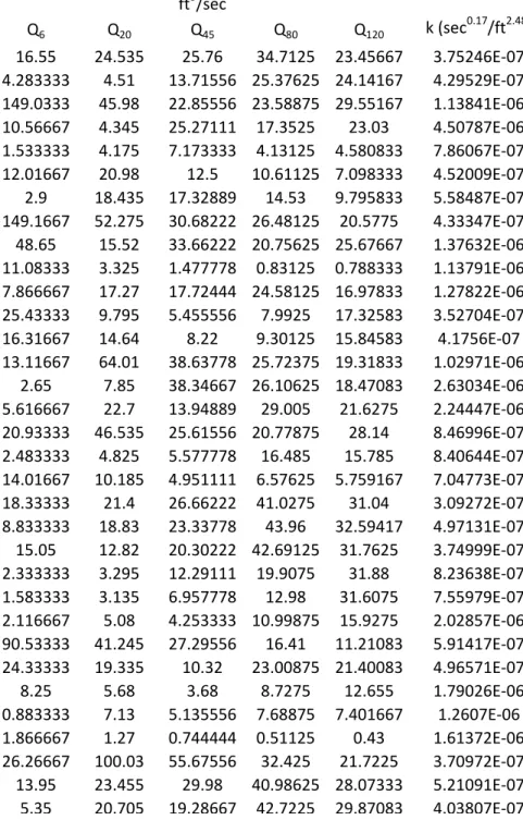
Selecting of past discharge Q N and k of each recession event
Calculating the Q avg by observing the trend of Q N
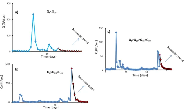
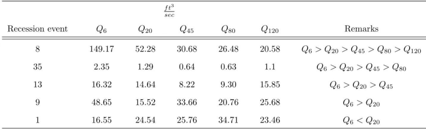
In such a case, the past stream flow from days 2 to 120 contributes to the recessional stream. In such a case, the past stream flow from days 2 to 80 contributes to the recessional stream. In such a case, the past streamflow from days 2 to 45 contributes only to the recessional stream.
In such a case, the past flow from days 2 to 6 contributes only to the recession flow.
Performing the linear regression analysis (ln converted linear regression anal-
Selection of regression coefficients corresponding to high strength of determi-
For all basins (λavg, k0avg) during the calibration period were shown in 9−10 columns of theSM−1 given at the bottom.
Calculating the Q avg for predicting the recession flow during the validation
Choosing the formula for predicting the dry weather flow (recession flow)
Suppose that if the recession or dry weather period lasts for a longer period, the dry weather flow can be predicted even without using the initial discharge, using the following formula. In our case, due to the availability of initial discharges during the validation period (second half of the data), recession flows were predicted using both equations 5.2 and 5.3.
Evaluating the model performance after calculating the dry weather flow
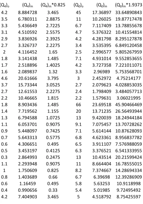
In the figure 4.5, (Q4)o=observed current flow of each recession event from day 4 without considering the initial discharge; (Q4)m=predicted streamflows of each recession event from day 4 without considering the initial discharge; (Q0)o=observed streamflows from each recession event from day 2 considering the initial discharge; (Q0)m=predicted streamflows from each recession event from day 2 considering the initial discharge. In this study, dry weather flows were predicted using the above formulas and the model performance was checked using various model evaluation statistics such as coefficient of determination (R2), NSE, PBIAS (percentage bias), RSR (RMSE - standardization ratio). For the later case, the model underestimates the observed flow by a factor of 1.9373 so all the predicted streamflows are multiplied by 1.9373 to remove the bias error.
For reference purposes, the first 29 days of observed and predicted streamflows are shown in Figure 4.6 only.
Relative gravity observing procedure
Station topography details and magnitudes of corrections for elevation and latitude . 37
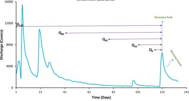
From here, recession event means it excludes two days, including the recession peak. Due to the high variability in the individual segments of the recession, it was calculated separately for each recession event. The prediction of streamflow after the peak of the recession curve is mainly influenced by the fact that the variation of a basin is limited.
Even without knowing the initial flow, it is possible to predict in advance the dry weather flow from the fourth day of the recession event using equation 5.3.
Anomaly of recession coefficient k with cumulative past discharge from a fixed reference 40
To calibrate recession parameters, individual recession events were selected from half of the available data. Sok values were calculated for all recession events using non-linear regression analysis after determining the α pool as the median α distribution of individual recession events. The presented α values of all basins were listed in column 8 of the attached supplementary material.
This type of improved relationship was observed in 74% of the total basins and the improvement in coefficient of determination values for all basins is reported in column 7 of the supplementary material provided.

Comparison of Bart’s approach and our approach
Correct choice of time step in the recession analysis can be one of the reasons which can be assumed to distinguish between R2P W Y and Ravg2 values. Also, the time step is strongly affected by precession and noise involved in the data [14]. The Institute of Hydrology (1980) suggested a time step of 2 days to account for precession of the data and the exclusion of multiple recession events of shorter duration in the case of longer time steps.
This was mainly to avoid the possibility of overriding basin properties in terms of smaller time step recession events [5].
Prediction of dry weather flow
For calibration using first half of data, validation using second half of data; for the same 3 cases, (d), (f), (e) represent scatterplots of predicted recession flows using initial discharge and observed recession flows. 03114500 the scatter plot of predicted streamflows (Qmod) and observed streamflows (Qobs) for the 3 cases (1. Model testing with first half of the data;. For the basin with USGS id:02182000 except in 3rd case, both the coefficient of determination values (one for the prediction without considering the initial discharge and the other considering the initial discharge) were observed to be almost the same, indicating that all the predicted streamflows were only function of k, while for the others comes with USGS id : 03114500 a significant difference between both coefficient of determination values was observed.
For the same forecast cases, the scatter plot of the forecast and observed recession flows for the basins was shown in the following Figures 5.9 and 5.10, respectively.

Removing the bias error in the predicted dry weather flows
Evaluation of model
Similarly, columns 14−15 indicate the unbiased, biased NSE values in which streamflows were predicted using the initial discharge. Similar model was tested using the whole data and the corresponding unbiased and biased NSE values are shown from columns 16-19 of the supplementary material provided (for the prediction without using initial discharge and using initial discharge ). Columns 20−21 indicate the unbiased and biased NSE values of predicted streamflows during the second half of the data.
Columns 20−21 of the supplementary material provided indicate the unbiased and biased NSE values for which the forecast streamflow was from the 4th day of the recession.
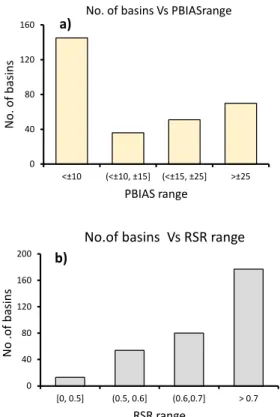
Cumulative frequency curves of model evaluation statistics
The above values correspond to predicted recession currents without using initial discharge and observed recession currents during the second half of the data with calibrated values from the first half of the data. The above values correspond to predicted recession currents without using initial discharge and observed recession currents during the second half of data with calibrated k values from the first half of the data. Above values correspond to predicted recession currents without using initial discharge and observed recession currents during the first half of data with calibrated values from the same data.
The above values correspond to predicted recession currents using initial discharge and observed recession currents during the second half of the data with calibrated values from the first half of the data.
Interpretation of relative gravity results
- Spatial variation of raw and corrected gravity residual
- Nature of gravity corrections in this study
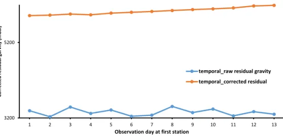
- Temporal variation of raw and corrected gravity
- Major factors in causing the variability of residual gravity
Thus, due to its significant influence, variation in moisture emerges as the strongest factor in causing the variability of gravity values at the microscale. So also at the micro scale it is concluded that the gravity values can be correlated with the variation of moisture and can be used to predict the fluctuations in storage. Relative gravity meters provide the difference in gravity values at a reference point and a target location.
So fluctuations in moisture content are reflected in gravity values corrected for other factors.
Conclusions
To test the utility of using microscale gravity variability as a tool in hydrologic modeling, spatial (at 12 stations) and temporal (3 months during the monsoon) gravity values were observed with a Scientrix CG-5 relative gravimeter. Our micro-scale study reveals that micro-scale gravity studies also aid in hydrological modeling. From the variation of gravity results over a 3-month period, it was determined that moisture variation was the strongest factor in causing gravity variability.
So our future work will be on distinguishing the effect of surface as well as subsurface moisture on the variation of microscale gravity values.
Limitations of work
For gauged basins, attempts have also been made to identify the dominant watershed characteristics that influence the prediction of dry weather flows. Thus, our future study will focus on optimizing the relationship between the model evaluation parameters of the measured basin and the comparable catchment characteristics of the unmetered basin. We found that investigating recession parameters with separated prior streamflows contributing to storage during that recession period plays a crucial role in better predicting k. As a result, the proposed algorithm can be used as a surrogate for predicting recession flows. of watersheds that are less or not affected by human extraction.
I = Validation using data from the second half; all model efficiency parameters are inclusive of bias error; j = Validation using data from the second half; all model efficiency parameters are exclusive of bias errors. A Geologic Framework for Interpreting the Low-Flow Regimes of Cascade Streams, Willamette River Basin, Oregon.
![Table 2.1: General recommended performance ratings for streamflow prediction corresponding to monthly time step (adapted from [18] )](https://thumb-ap.123doks.com/thumbv2/azpdfnet/10482844.0/24.892.151.874.229.388/general-recommended-performance-ratings-streamflow-prediction-corresponding-monthly.webp)