To the best of my knowledge, no part of the work reported in this thesis has been presented for the award of any degree at any other institution. In the last section we will talk about the outline of the thesis and our contribution.
MODEL OF COMPUTATION
Model of Computation
The Problem Statement
If the element is part of the subset S that is given to store, then we store one for that element. On the other hand, if the element is not part of the given subsets to store, then we store zero for that element in the table.
Definitions
Now, given a query element x∈ U, we look in the table and say that the query element is part of the given subset to be stored if and only if the stored bit returned is one. Although the number of queries required in this solution is one, the amount of our space, i.e.
HISTORICAL NOTES
Historical Notes
Thesis Outline and Contributions
This chapter starts with some simple explicit non-adaptive upper bounds, and ultimately uses them to obtain an explicit non-adaptive scheme that uses slightly fewer bit probes and slightly more space than existing state-of-the-art results. Furthermore, we investigate an explicit non-adaptive (4, m,O(m2/3),4) scheme, and further improve it to store the subset of up to five with the same amount of space.
THESIS OUTLINE AND CONTRIBUTIONS
Introduction
REVISITING TWO ADAPTIVE BITPROBE SCHEME
Revisiting Two Adaptive Bitprobe Scheme
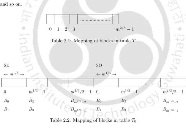
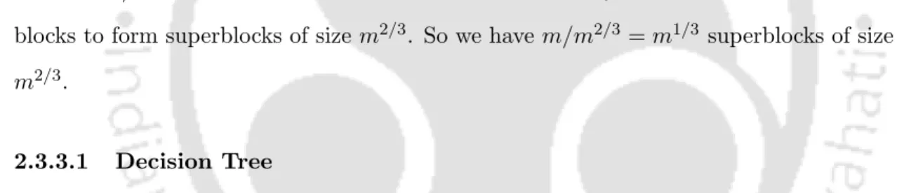
Further, we send the rest of the blocks to tableT1 and store its characteristic vector there. Further, the rest of the blocks are sent to TO, with all bits set to zero.
ON THE THREE ADAPTIVE BITPROBE SCHEME
On the Three Adaptive Bitprobe Scheme
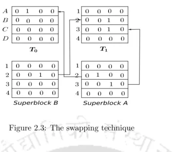
Now, since each superblock has a block with space in table A and table B, we send a block from remaining superblocks with an element(s) in it to table A. We select a block from the remaining blocks that have an element in itself and maps it to the first table of type T, and we map the block originally mapped to that location to table A.
Conclusion
The correctness of the scheme rests on the fact that blocks containing elements from the set given to be stored are always given a separate place in one of the tables at the leaf. Additionally, blocks that contain no elements from the set given to be stored are always given a location in table B where each bit is set to zero.
Introduction
Non-adaptive Upper Bounds
NON-ADAPTIVE UPPER BOUNDS
There is an n+3 probe explicit non-adaptive scheme which stores an arbitrary subset S of size at most 2n+1, from a universe U of size m and requires O(n1.5m2/3) amount of space. On the contrary, if the query is made from the block with at most n elements, it ignores the bit returned by tables that store characteristic vectors of blocks with at least n + 1 elements, and answers the query depending on the last + 1 queries.
Conclusion
Furthermore, we use Theorem 3.1 to map the blocks that have the most elements from the set to be stored. If a query is made from a block that has at least n+ 1 elements, it ignores all tables except the table belonging to its rank, where its characteristic vector is stored.
Introduction
INTRODUCTION
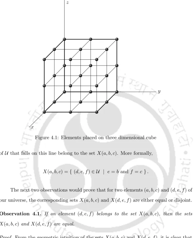
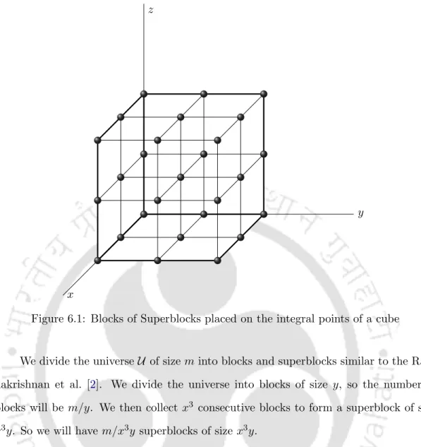
It uses Keshe's technique [18] of mapping the elements of our universe to the integral points of a three-dimensional cube and then looks at the projections of the various points onto the two-dimensional faces of the cube. Using this idea, we improved our non-adaptive scheme to store a subset of size five (n = 5) by using four non-adaptive bit probes (t = 4) and still using s = O(m2/3) bits of space.
Adaptive Scheme for n = 3 and t = 2
ADAPTIVE SCHEME FOR N = 3 AND T = 2
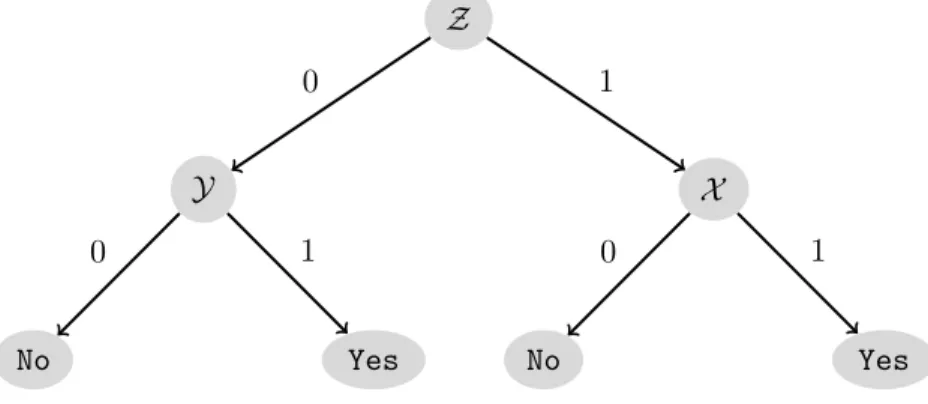
Case II(B) We now consider the second subcase, where the y-coordinate of the third element is different from the de-coordinate of the other two elements. Bits in table Z corresponding to the three members are set to 0, so the second query for all the members will be made in table Y.
A NON-ADAPTIVE SCHEME FOR N = 4 AND T = 4
A Non-adaptive Scheme for n = 4 and t = 4
Case II(A) – Let us assume that in the partition Z, the element (a4, b4, c4) is in one of the sets of the other three elements of S. Case II(B) – We now consider the scenario when the element (a4, b4, c4) is not in any of the groups of the other three elements in the Z partition.
In table C, the bits corresponding to the first four elements, namely C(ri, vi) where 1 ≤i≤4, are set to 1 and the rest to 0. As usual, in table D only the bits corresponding to members of S are set to 1. In table B, bits of members of S are set to 1, and the rest of bits to 0.
Finally, in table D, the bits of the members of S are set to 1, and the rest to 0. In this case, the bits corresponding to the members of S are set to 0 in table A, and those in table B are set to 1.
CONCLUSION
Conclusion
Introduction
INTRODUCTION
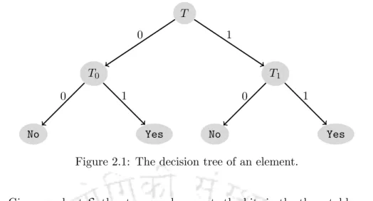
The scheme presented in this paper is an adaptive scheme that uses two bit probes to answer membership queries. We now discuss in detail the bitprobe model in the context of two adaptive bitprobes. Given a subset, the storage schema sets bits in the three tables so that member queries can be answered correctly.
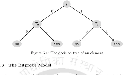
If the stored bit is 0, the second query is made on table T0, otherwise it is made on table T1. If the answer to the second question is 1, then we declare that elementix is a member of S, otherwise we declare that it is not.
Our Data structure
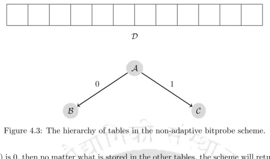
The data structure in this model consists of three tables –T, T0 andT1 – arranged as shown in Figure 5.1. By slightly misusing the notation, we will use the same symbols to represent the bits stored in those locations. The flow of the query schema is traditionally captured in a tree structure, the so-called schema decision tree (Figure 5.1).
OUR DATA STRUCTURE
So we can store the four non-empty blocks in table T0, and all empty blocks in table T1. In this scenario, the four non-empty blocks can occupy four different coordinates of the grid. We now look at the assignment of the blocks that fall on the two non-empty lines.
Case IV(A): Let us consider the scenario when three of the non-empty blocks coincide. The rest of the blocks of the line ls3(x3, y3) can now be stored in table T1 without conflict.
CONCLUSION
Conclusion
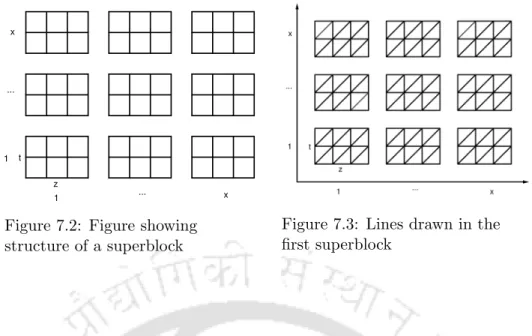
The technique used is to arrange the blocks of a superblock in a two-dimensional grid and group them along lines. We believe that this technique can be extended to store larger subsets by extending the idea of an arrangement in a two-dimensional lattice to arrangements in three and higher dimensional lattices.
Introduction
OUR DATA STRUCTURE
Our Data Structure
We send the block with element n2 to table T0 and all blocks that lie on the line containing this block table T1. We send the block with element n2 to table T0 and all blocks that lie on the line containing this block table T1. We send the block with element n4 to the table T1 and the empty blocks that lie on the line containing this block to the table T0.
Further, we send the empty blocks of the line which contain block with element n5 to table T1. We send the block with element n5 to tableT0, and all the empty blocks on the line containing this block to table T1.
CONCLUSION
Conclusion
Introduction
INTRODUCTION
Lower Bound
LOWER BOUND
If f is a member of UB(e) such thatC(f)∩ S={f}, then all other members of C(f) must be stored in tableB. If e, a member of S, is stored in table B, then Observation 7.2 tells us that all members of UB(e) must be stored in table C. Ifx ∈ A(e), since e is stored in table B, so that all elements of A(e), including x, must be stored in table B.
If x∈ B(e)\ {e}, and ase has been stored in table B, observation 7.2 tells us that x should be stored in table C. If/S contains and x, and we store in table B, observation tells 7.2 tells us that z∈ UB(e) must be stored in table C, and as x ∈ C(z), observation 7.5 tells us that x must be stored in table B.
OUR DATA STRUCTURE
Our Data Structure
In this case, we send all blocks with elements to tableT0 and all empty blocks to table T1. In this case, we send the blocks with elements n4 and n5 to table T1, and all the empty blocks lying on the dashed line containing these blocks to table T0. In this case, we send the block with element n1 to table T0, and rest all the blocks lying on the dashed line containing this block to table T1.
Next, we send the block with element n4 to table T1 and all empty blocks lying on the dotted line containing this block to table T0. In this case, we send the block with element n1 to table T0 and all blocks lying on the dotted line containing this block to table T1.
Conclusion
Appendix A
APPENDIX A
We will first calculate the value of the following expression. collect over the sets of B). Here the sum of the coefficientsscX ism and the number of terms, which is the same as the number of sets of B, iss.
Appendix B
APPENDIX B
In this case, we send the block with element n1 to table T0, and rest all the blocks lying on the dashed line containing this block to tableT1. In this case, we send the block with element n2 to table T0, where all the blocks lie on the dashed line containing this block, to table T1. Further, we send the block with element n2 to table T0, where all the blocks lie on the dashed line containing this block, to table T1.
We send the block with element n5 to table T0, and all the blocks lying on the dashed line containing this block to table T1. In this case, we send the block with element n1 to table T0, and all the blocks lying on the dashed line containing this block to table T1.
Appendix C
APPENDIX C
In this case, we send the block with element 1 to the T0 table and all the blocks that span the row containing this block to the T1 table. We send the block with element n3 to tableT0 and all empty blocks that span the row containing this block to table T1. We send the block with element3 to tableT0 and all empty blocks that span the row containing this block to tableT1.
Further, we send the block with element1 to tableT0, and all the blocks on the line containing this block to tableT1. We send the block with element n5 to tableT1, and all the blocks on the line containing this block to tableT0.