It is certified that the work contained in the thesis titled "Effect of Disturbance and Mixing of Different Species on the Collective Behavior of Self-propelled Particles". However, the collective dynamics of SPPs with inherent perturbations in the system are rarely studied.
Literature Review
Different collective properties were observed in the study of the VM with topological interactions (occurring between a fixed number of neighbors) [97]. The study of geometric properties of the different patterns is also investigated using cluster size analysis in recent works [120, 121].
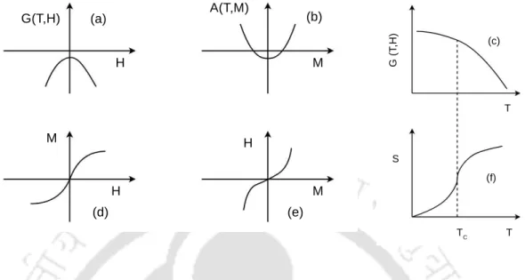
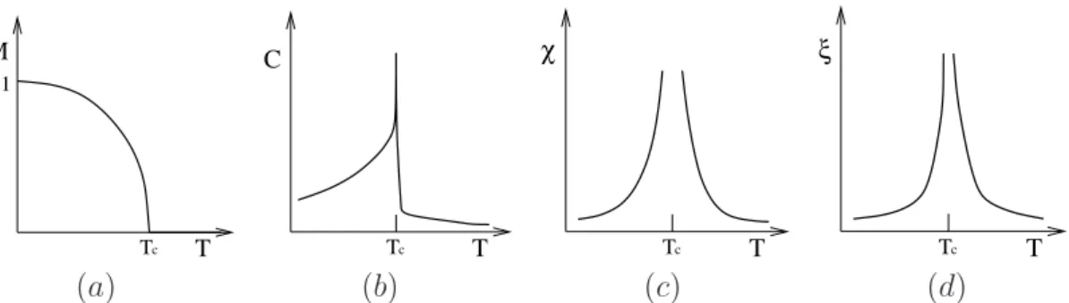
Phase transition and its characteristic features
In a first-order phase transition, there is usually a radical change in the structure of the material. Continuous Transition: For a second-order continuous transition, the two free energy curves meet tangentially at the critical point.
Spin Models
The Hamiltonian for such a 2d XY model with nearest-neighbor interaction J and no external field is given by. In 2d, however, the XY model undergoes a Kosterlitz-Thouless transition in which no long-range order is present in the system.
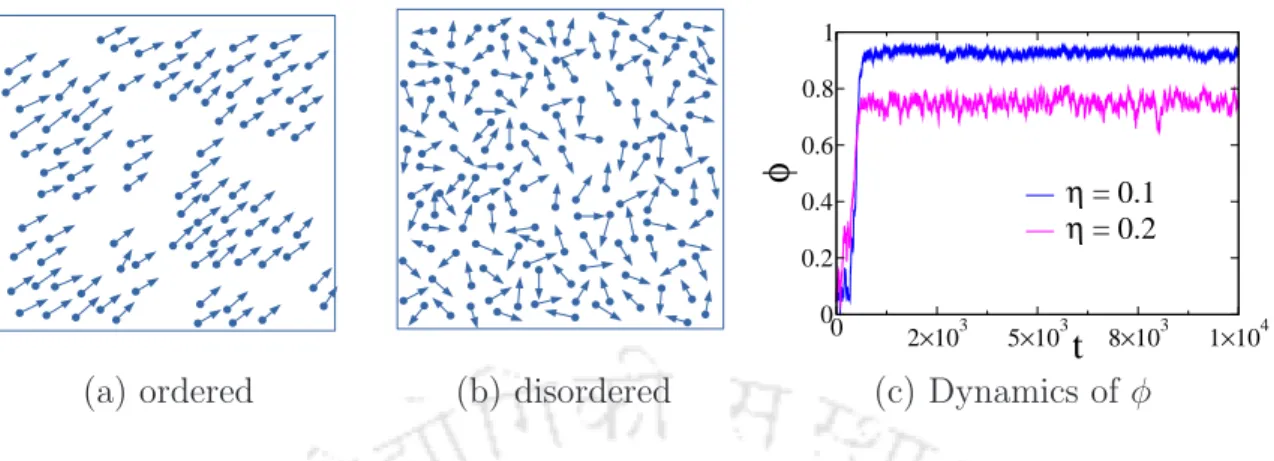
Vicsek Model
While alignment interactions between particles produce such information, the angular noise present in the system destroys it. There is only one conservation law in VM: conservation of the total number of particles.
Motivation and Plan of thesis
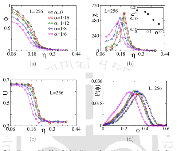
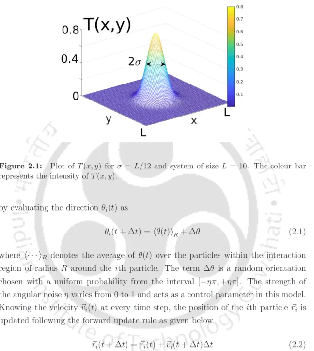
The effect of perturbation on VM is studied, varying the scalar noise η and the perturbation strength α. It is then intriguing to study the effect of perturbation on the formation of density bands as well as the natural phase transition.
Results and Discussion
- Methodology and Algorithms
- Finite size scaling
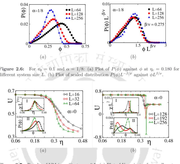
- Results at v 0 = 0.1
- Results at v 0 = 0.5
- Results at v 0 = 1.0
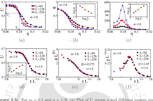
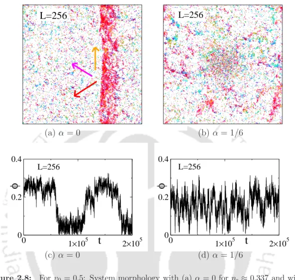
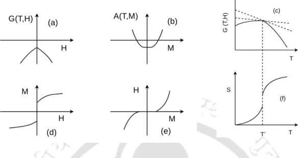
In fig. 2.5(b), order parameter φ is plotted against η for different L using the same symbol set in Fig. 2.5(a). Susceptibility χ is plotted against η in Fig. 2.5(c) for different L using the same symbol set in fig. 2.5(a). The nature of the transition is found to be independent in the wide range of the perturbation strength α.
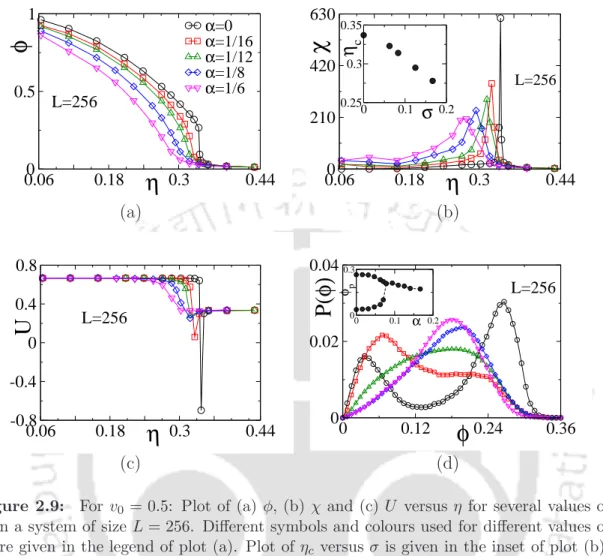
The corresponding steady-state dynamics of the order parameter for the system with α= 0 is given in Fig.2.8(c) at η≈ηc. The trapping perturbation is not enough to destroy the formation of the moving band in the system.
Summary and Discussion
Even with a perturbation strength α= 1/6, the moving band in the system persists with a slight distortion around the central zone of the trapping perturbation. In the presence of trapping disorder, the value of crossover system sizeL∗α(ρ0, v0) increases and becomes larger than L∗(ρ0, v0), that of without disorder. Furthermore, the continuous transitions observed in the VM with disturbance are characterized by the same critical exponents of the VM without disturbance forL < L∗(ρ0, v0).
For the systems larger than L∗α(ρ0, v0), the transition remains discontinuous even in the presence of perturbation. Patterning and phase transition in the collective dynamics of a binary mixture of polar self-propelled particles.
Results and Discussion
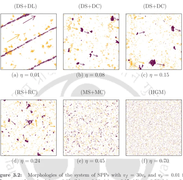
Collective Patterns
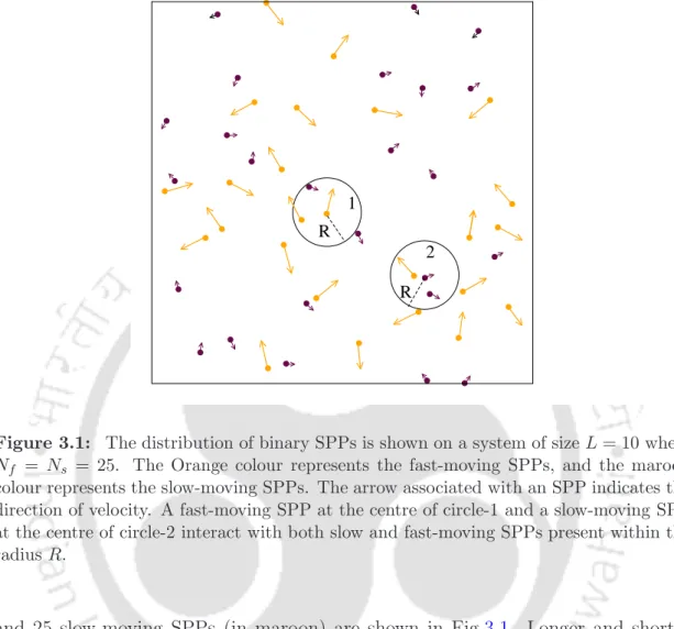
On the other hand, the slow-moving SPPs move on a narrow track in the same direction (indicated by the maroon arrow) as the clusters of fast-moving SPPs. With the increase of η, the focused clusters of fast-moving SPPs appear a bit scattered, while the slow-moving SPPs form clumps (or compact clusters) that still move in the same direction of DS of the fast-moving SPPs. Whereas in the BM, in the presence of alignment interaction only, the lane pattern through the slow moving SPPs occurs for very little noise.
Similar ordered phase (at low noise) patterns also appear in the cases of higher velocities of the fast-moving SPPs such as vf = 50vs and vf = 150vs with vs= 0.01. In the inset of (d), P(θ) is plotted for η= 0.16 with the same symbols and colors for the fast and slow moving SPPs.
Phase transition
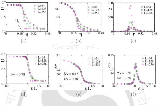
Similarly, the fourth-order Binder cumulant for the full system U and for partial systems Up is defined as,. If the transition between orientational order and disorder is continuous, the finite size scaling (FSS) relations of the above parameters can be given by the equilibrium thermal critical phenomena as The derivative of U(η, L) with respect to η follows the scaling relation, where the primes on U and U0 denote their derivatives with respect to η.
Since the system exhibits the coexistence of two phases, the distribution of the order parameter P(φ) would be a bimodal distribution for a discontinuous transition.
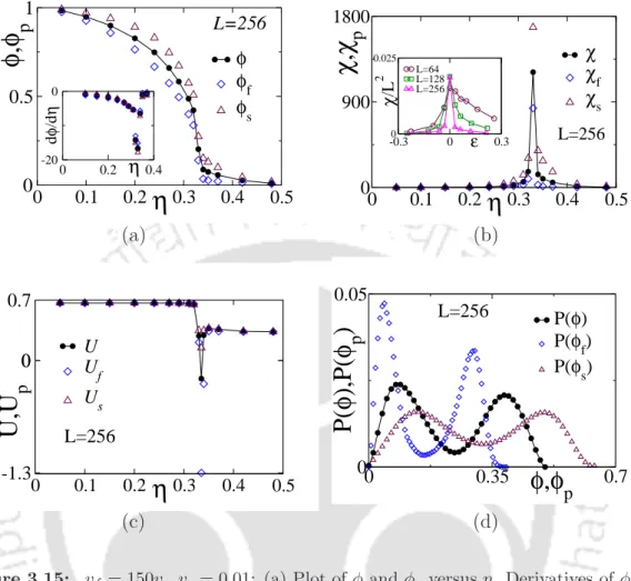
Derivatives of φ and φp with respect to η are shown in the inset. c) Plot of U and Up versusη. Thus, the order parameter of a specific type of SPPs is highly influenced by the movement of other types of SPPs in the BM. It is important to note that in the VM with monodispersed SPPs there exists a crossover system size L∗(ρ0, v) above which the transition is discontinuous.
Such discontinuous transitions are characterized by the appearance of dense traveling bands in the system. Although the nature of the transition in the whole system as well as in the partial systems remains the same as in the low-speed VM, the critical exponents are different.
The order parameter φ of the whole system and the partial systems parameter φp are plotted against η in Figure 3.9(a). Slow SPPs appear to have a significant influence on the non-formation of traveling bands with fast moving SPPs as well as on the nature of the phase transition. It is interesting to note that both types of SPP maintain the same nature of the phase transition in the BM.
Now we perform the FSS analysis in this case to extract the values of the critical exponents. The values of the critical exponents are reported in table.3.1 and compared with the others.
Moreover, since the critical exponents for the case vf = 50vs differ from the case vf = 30vs, the universality class of BM depends on vf for a fixed vs. It seems that, in the case of vf = 100vs (vs = 0.01), the order parameter distribution differs from the unimodal distribution. In this case, a dense traveling band of fast-moving SPPs appears in the system near the transition η ≤ηc with the directed clusters (DC) of slow-moving SPPs (Figure 3.14(a)).
Whereas, for η > ηc, random clusters of fast-moving and random clumps of slow-moving SPPs, RS+RC phase occurs in the system.
- Effect of interaction radius R
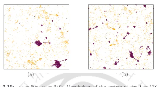
Even more interesting is what these two phases are for slow SPPs. Figure 3.16(a) shows a dense traveling band of fast-moving SPPs and clumps of slow-moving SPPs. However, in Fig. 3.16(b), the dense traveling band of fast moving SPPs disappears and clusters of slow SPPs begin to move randomly in the system.
The slow moving SPPs therefore follow the direction of movement of the moving band of the fast moving SPPs. Consequently, the clumps of slow-moving SPPs and the clusters of fast-moving SPPs move randomly.
Summary and Discussion
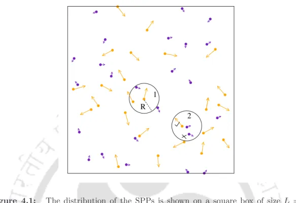
The adapter SPPs do not interact with each other, but adopt the velocity orientation of the usual SPPs through local interactions. However, the usual SPPs interact with themselves as well as with the adapters. A mixture of usual SPPs with adapter SPPs is modeled over a two-dimensional square box of linear size L with periodic boundary conditions.
If N0 is the number of common SPPs and Na is the number of adapters, then N0 =Na =N/2 where N is the total number of SPPs in the system. The distribution of randomly oriented 25 common SPPs (in orange) and 25 adapters (in indigo) is shown in Fig.4.1.
Results and Discussion
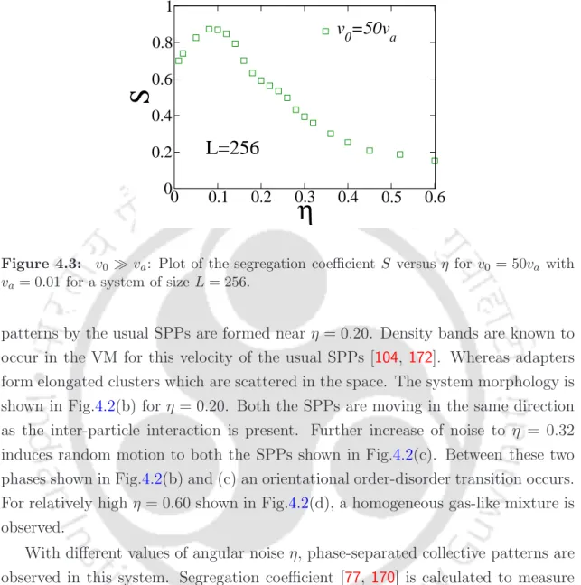
Density bands are known to appear in VM for this rate of conventional SPPs [104, 172]. The order parameter φ of the whole system and the partial systems parameter φp are plotted against η in Figure 4.4(a). In this model, the value of the order parameter of conventional SPPs (φ0) is higher than the order parameter of adapters (φa).
The derivatives of φ and φp with respect to η are plotted in the inset of Fig.4.4(a) and minima of the plots at the transition noise ηc ≈ 0.27 are observed for systems with the usual SPPs as well as for the whole system. Similarly, the fourth-order Binder cumulant for the whole system and that of the partial systems is defined as, .
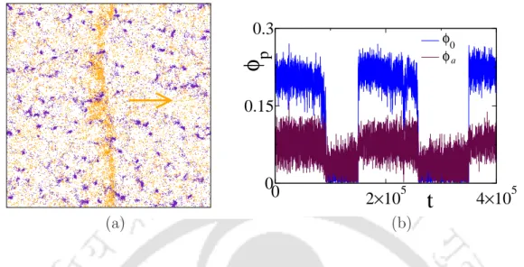
Below we explain the situation by studying the time evolution of the system morphology in the transition region. The density band of ordinary SPPs is moving in a certain direction (shown by the orange arrow). The steady state dynamics atη=ηc of the order parameters is given in Fig.4.7(b) where the values of both φ0 (blue) and φa (brown) fluctuate between the two phases in a synchronized manner.
The higher value of φ0 corresponds to the presence of the traveling band (an ordered phase) and the lower value of φ0 corresponds to the disappearance of the traveling band (disordered phase). This keeps the speed of the usual SPPs v0 and that of the adapterva both high and beyond, va > v0.
The Model
In this section, we consider a situation where orientational adapters move at higher speeds than ordinary SPPs. Apart from the speeds, all other characteristics of the common adapters and SPPs remain the same, as mentioned in part-I.
Results and Discussion
In this case, the speed va of adapters is almost the same as the usual SPPs. The cumulants for the usual SPPs (U0), for adapters (Ua) and for the whole system (U) all show a sharp negative drop at the transition. This is expected as the adapters follow the usual SPPs; they move in the direction of the density band.
Moreover, their speed is similar to ordinary SPPs; they also form a dense band pattern next to ordinary SPPs. The situation will be different for a much higher speed of adapters with the same speed of ordinary SPPs.
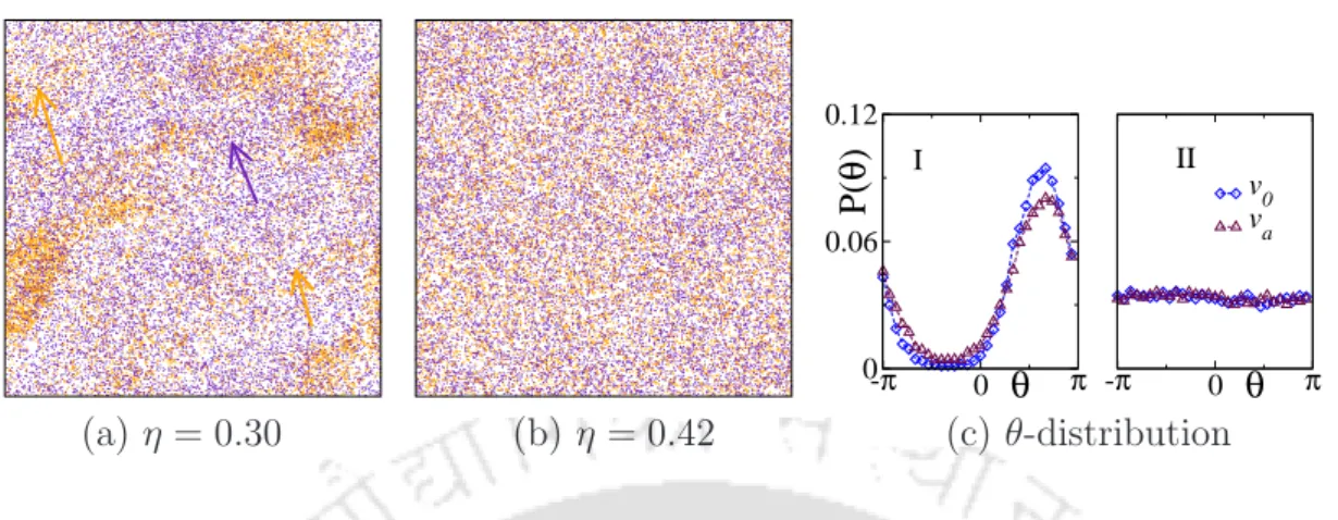
During the transition, at η = 0.30 shown in Fig. 4.13(a), less dense large clusters of usual SPPs are observed with small clusters of adapters, and they are aligned in the same direction (shown by arrow). In this case, adapters move at much higher speed and cannot be flocked with the usual SPPs. It appears that as the usual SPPs interact with the adapters, randomness enters into the alignment of the usual SPPs.
Observations show that when va is relatively less as va = 1.2v0 with v0 = 1.0, a sudden jump in theφt arises and the positions of the jump from the implementation of the forward and backward simulation schemes are different. Then, for a sufficiently large value of va = 7.0v0, the variation of the order parameter with respect to η becomes reversible,.
Summary and Discussion
For adapter speed va = 1.2v0 and v0 = 1.0, both adapter and ordinary SPPs form dense traveling bands in the system. The nature of the transition is further confirmed by the existence of hysteresis in the order parameter under a continuously varying noise field. Such a mismatch in orientations between adapters and SPPs introduces additional fluctuations in the system.
For the adapter velocity va = 1.2v0 and v0 = 1.0, both adapters and the usual SPPs form tight motion bands and move in the same direction. In the ordered phase, the flocks of usual SPPs form directed clusters, and the adapters form relatively less directed clusters.