27 2.3 Comparison of SVLT performance with that of EYM, USA and. 27 2.4 Comparison of SVLT performance with that of EYM, USA and.
Matrix estimation using SVD
Data model
We can think of it as the source of interference in the columns (rows) of the data matrix X. To address this, the correlation between the columns (rows) e of the underlying signal matrix of the noisy data matrix X.e Therefore, it is interesting to see the effect of noise on the SVD of
Spectral regularization
Spectral estimator of a matrix
Random matrix theory
Empirical singular value distribution
Therefore, it is important to study the effects of the noise matrix on the signal SVs as well as on the corresponding singular vectors. Furthermore, it can be seen from (1.17) that the data SVs are always positively biased with respect to the signal SVs, confirming the “shrinkage toward zero” nature of the shrinkage estimators.
An asymptotically optimal shrinkage estimator
Often, data SVs greater than β+ are considered active SVs, and the number of active SVs is taken as an estimate of the rank, i.e. r∗ = PL. Contrary to (1.15), we show that it is possible to obtain the optimal estimate by shrinking the data SVs while the singular vectors remain unchanged.
Stein’s unbiased risk estimator of the MSE
For the same, the value that achieves the minimum of SURE is taken as the optimal parameter value, thus SURE acts as a surrogate for MSE. In the following, we discuss about SURE and its use in determining parameters for spectral estimators.
Optimal shrinkage using the RMT and the SURE
Progress and challenges
Problem formulation and objectives
However, it could not achieve the optimal truncation of the SVHT and the optimal shrinkage of the SVST at the same time. Motivated by the above challenges, we aim to design an estimator that completely decouples the truncation and the shrinkage of the SVs so that they can be controlled separately.
Contributions of the thesis
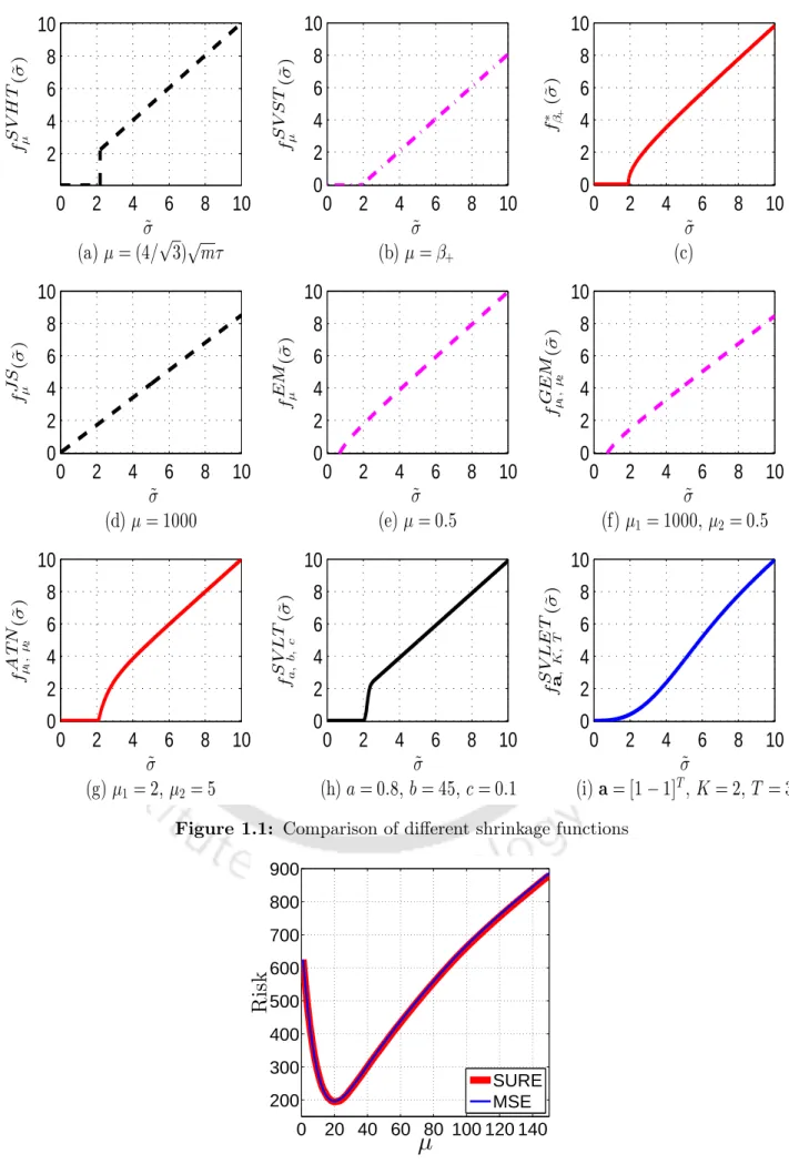
In Figure 1.1, the proposed shrinkage functions are compared with the various existing shrinkage functions. We wish to further explore the proposed SV shrinkage-based estimators for signal decomposition tasks involving electrocardiograms (ECG), photographic images, and magnetic resonance (MR) images.
Organization of the thesis
SURE based rank estimation methods
According to the EYM theorem, for a real matrix The rank estimation methods discussed above have been used to provide ranking contrast.
Drawbacks of the existing rank estimators
Proposed method
Experimental results and discussion
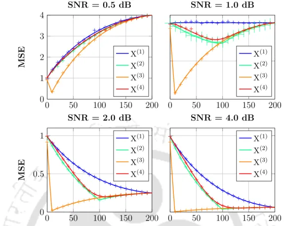
- SURE for SVLT vs. MSE
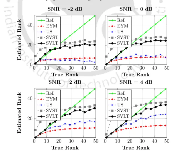
- Rank estimated by SVLT vs. true rank
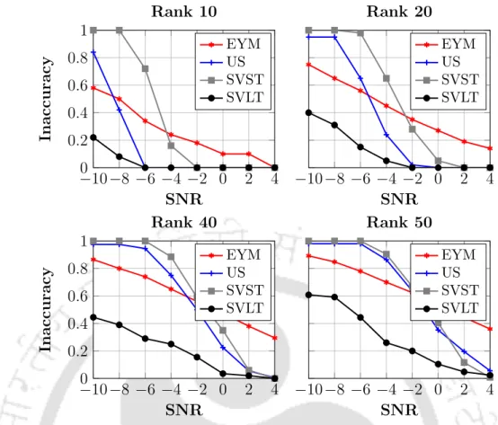
- Quantitative performance of the SVLT based rank estimator
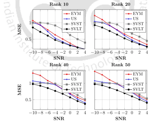
- Quantitative performance of the SVLT based matrix estimator
In this experiment, we compare the quantitative performance of the SVLT-based rank estimator with existing methods. The SVLT method consistently outperforms contrast methods for low-level matrix recovery in terms of MSE.
Summary
In the SVST method, a sub-optimal trade-off is made between preserving the signal-dominant SVs and suppressing the noise-dominant SVs. This is due to the decoupling of the shrinkage and truncation achieved by using additional parameters in the proposed SVLT method.
Proposed method
Linearized shrinkage function
After that, in this paper, we adopt DOG as the basis for the linearization of the unknown shrinkage function. In Figure 3.1(d), a typical example of the proposed DOG-based shrinkage function is compared with some existing shrinkage functions.
Asymptotic behavior of the SVLET
Such an estimator is referred to as the bulk shrinker generated by SVLET in the rest of the thesis. In the asymptotic setting, the bulk shrink generated by SVLET obtains the true mean squared error estimator and it boils down to an optimal bulk shrinkage estimator.
Results and discussion
Selection of parameters
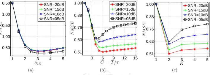
In each case, the average NMSE calculated over all possible rows of the underlying pure matrix is reported. Therefore, the choice of C = 10 and K = 2 is reasonable enough to be fixed in the rest of the experiments in this chapter.
![Figure 3.1: Comparison of existing singular value shrinkage functions. A typical example of (a) asymptotically optimal bulk-shrinkage function [1], (b) ATN [2] (µ 1 = 2.2, µ 2 = 5), (c) SVLT [3] (a = 0.8, b = 2.2, c = 0.1), and (d) proposed SVLET shrinkage](https://thumb-ap.123doks.com/thumbv2/azpdfnet/10540591.0/70.892.87.776.85.1091/comparison-existing-singular-shrinkage-functions-asymptotically-shrinkage-shrinkage.webp)
Matrix denoising performance
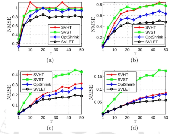
- Comparison with RMT based methods
- Comparison with SURE based methods
In Figure 3.2(a), the NMSE, averaged over all ranks and 1≤K ≤5, is plotted against different values of C. The reason behind this behavior is the sufficient fit of the shrinkage function in capturing the single value profile of the matrix of the original signal with only the parameter a.
Summary
The weight applied is proportional to the similarity in the environment and independent of the temporal location of the samples. The final estimate of the ECG signal is found by means of these estimates; thus further reduction in the additive noise is achieved.
Proposed ECG denoising method
SDM extraction
Blocks of samples that are marked with the same colors are similar and grouped into one SDM. The goal of this step is to find blocks such that their noise-free base counterparts are similar.

Noise filtering
- Denoising by thresholding of 2D DWT coefficients
- Denoising by singular values shrinkage estimators
Comparing Figures 4.2(a) and 4.2(b), it can be seen that the structural similarity in the SDM blocks is well preserved with the proposed shrinkage of the 2D DWT coefficient. It can be noted that the noise-free SDM by the SVLET method is smoother than that of the NLWT method.
Aggregation
At the end of this step, we obtain a denoised version of each SDM, which must be summed to obtain the final estimate of the ECG signal. In Figure 4.2(b) and (c), we show the denoised versions of a noisy SDM from the NLWT and SVLET methods.
Selection of parameters
- Block size and overlap
- Search window
- Block matching threshold and SDM size
- Hard-threshold for NLWT
- Order of linearization and transition parameter of the SVLET
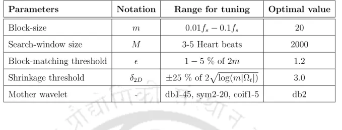
In the following, we discuss how the various parameters for the proposed methods are determined. This is done to meet the requirement of the spectral estimators used to degrade the SDMs in the proposed SVSE methods.
Experimental results
Performance measures
Evaluation on MIT-BIH Physionet database
Similarly, the fixed parameters of the SVSE methods are also set to the same test signal. To evaluate the noisy performance with the parameters chosen above, we chose different realizations of the noise at different SNR levels.
Evaluation on PTB Diagnostic database
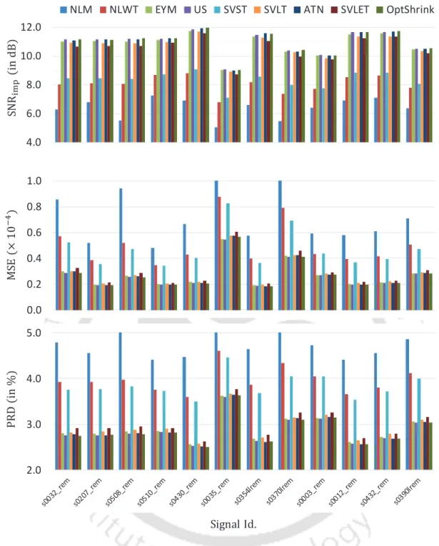
The biomedical signals contain a number of diagnostic features that must be visually inspected by physicians. When comparing with the noise-free signal, it can be seen that the signal denoised by all proposed methods is more similar to the clean signal than the noisy signal itself.
Discussion
The SVLET and RMT based OptShrink estimators perform closely in terms of the MSE and the PRD, while the latter outperforms the former in terms of the SNR improvement. This could be because the asymptotic assumptions of the RMT-based shrinkage method in SDM are sufficiently satisfied due to its inherent low ranking.
Summary
- Block matching based 3D filtering (BM3D)
- Higher order singular value decomposition based CF
- Weighted nuclear norm minimization (WNNM)
- CF with low-rank approximation
- Low-rank collaborative filtering (LRCF)
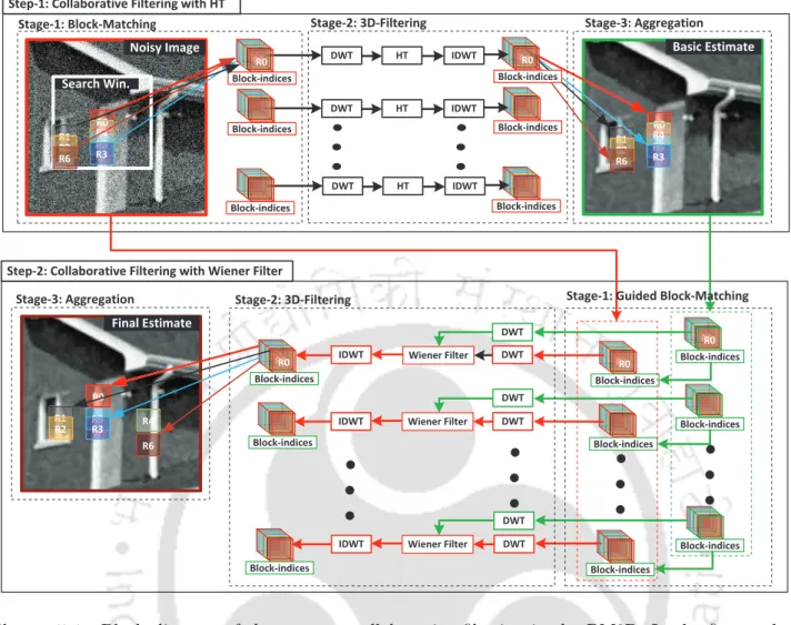
In the first step, the CF is done by hard thresholding the 3D DWT coefficients which yields a basic estimate of the underlying noise-free image. Note that in the first CF step of the BM3D, the block matching is performed on the noisy image itself.
Proposed methods
Denoising with FRIT in CF
Therefore, better denoising performance could be achieved using hard threshold values for the FRIT coefficients compared to the 2D DWT coefficients. It is noted that the attenuation using hard threshold values for 2D DWT coefficients results in blurring of the edge.
Denoising by matrix estimation in CF
Therefore, in the first step of CF BM3D, we replace the 2D DWT with FRIT while keeping the 1D Haar transform in the stacking dimension. Thus, using this baseline estimate, a refined image is obtained using the second CF step of BM3D.
Experimental set-up and parameter tuning
Parameters of the proposed CF methods
- Parameter tuning for the FRIT-CF method
- Parameter tuning for the SVLET-CF method
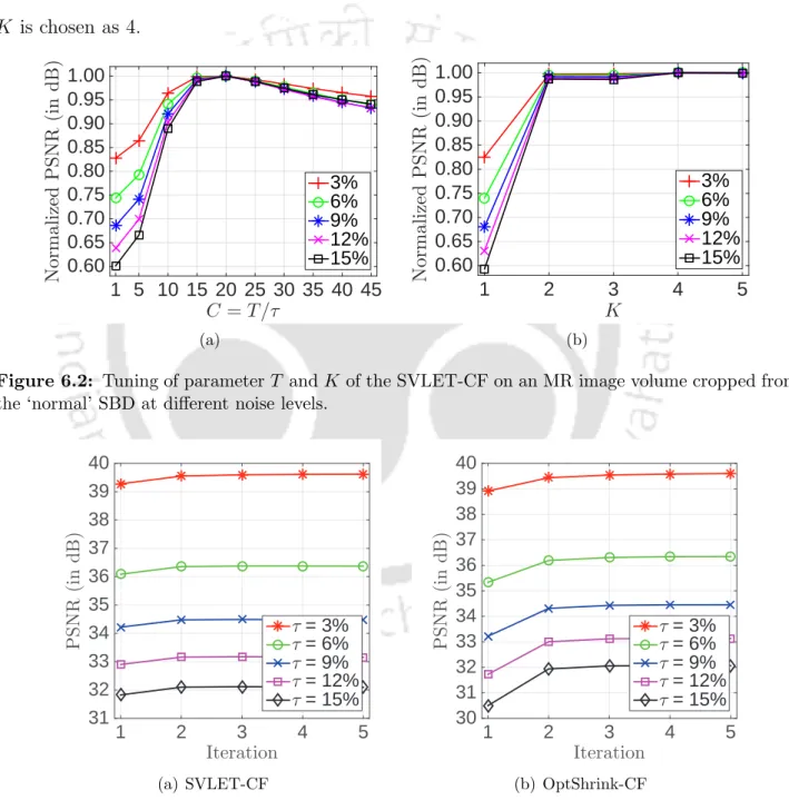
In the following, we describe the parameter space and the tuning of the key parameters for both the proposed FRIT-CF and SVLET-CF methods. a) Performance comparison in case of global processing. In Figure 5.8 we show the effect of iteration on performance of the proposed SVLET-CF method.
Results and discussion
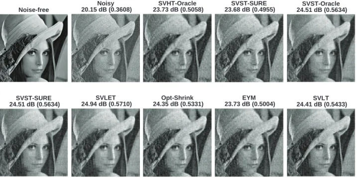
The overall performance of the FRIT-CF method is quite comparable to that of the BM3D method. The PSNR of the denoised image by the FRIT-CF is significantly higher than that of the BM3D method in the case of the Straw and the Grass images.
Summary
It is common to model the noise in the real and imaginary parts of the MR image as AWGN. In [123], a robust noise estimation method was proposed to automatically set the parameters of the combined local linear mean square error (LLMSE) filter and the anisotropic diffusion filter for denoising MR images.
Noise in MR image
Variance stabilization
From (6.3) and (6.4), it is clear that neither the mean nor the variance are independent of the noise-free underlying signal y.
Proposed MR image denoising method
Block grouping
A set of similar blocks is formed for each of the reference blocks using block matching. For each of the reference blocks, the m most similar vectorized blocks including itself are selected to form an SDM of size 1n2n3×m.
Noise filtering
- Noise filtering by SVLET
- Noise filtering by OptShrink
To exploit the non-local correlation of small 3D blocks of the MR image, these are grouped together. In our earlier explorations, it was also found to result in a competitive screening performance compared to that of the SVLET method.
Aggregation
Experimental set-up and parameter tuning
Performance measures
It is clear that a better denoising method should result in a higher PSNR value. ii) Structural Similarity Index Measure (SSIM) [145]: In an image, the SSIM calculates the properties of the human visual system and measures the structural similarity of the damped image with the underlying noise-free image. The SSIM is generally accepted as a better performance measure than the PSNR in terms of visual quality.
Selection of parameters
For this, we apply one-step denoising (which includes block clustering, batch denoising and clustering) to an MR image volume derived from the above database at different noise levels. In Figure 6.2(a), the normalized PSNRs are plotted against C, where T =τ C, for denoising a noisy MR image at different noise levels.
Effect of iterations
Results and discussion
Summary
The motivation behind the first one is to improve the estimation accuracy of the existing shrinkage estimators by decoupling the truncation and the shrinkage of SVs. The experimental study of the SVLET has shown that it is one of the fastest methods.
Future directions
Philips, “Image denoising using projected Gaussian scale mixtures,” IEEE Transactions on Image Processing, vol. Zeng, “Image fusion using higher order singular value decomposition,” IEEE Transactions on Image Processing , vol.