148 Figure 6.29: Crack probability functions for the Shaft-II with two cracks (one near . 13th measurement location and the other near 7th measurement location, first set of measurement). 149 Figure 6.30: Crack probability functions for the Shaft-II with two cracks (one near . 13th measurement location and the other near 7th measurement location, second set of measurements).
Importance of Study
The present chapter discusses the various causes for the development of cracks in machine elements and also the advantages and limitations of various crack detection techniques. A summary of the thesis is provided with a brief description of the content of each chapter.
Background and Literature Review
Background
The prediction of remaining life can be done using fracture mechanics and fatigue life analysis, which is a forward problem, while the problem up to level 3 is a reverse problem. Thus, the problem of remaining life prediction can be treated separately up to level 3.
Literature review
They represented local buckling due to the presence of a crack with a 6×6 matrix, including torsion. The opening and closing of the crack depends on the bending stresses in the shaft.
Present Work
Next, experimentation on real cracked shaft was done for the verification of the proposed algorithm. A scheme is proposed to reduce the effect of measurement noise in the performance of the algorithm.
Organization of the Thesis
The open crack pattern is provided and additional flexibility is gained due to the crack. Finally, the equations of motion of the intact shaft as well as the cracked shaft are obtained.
Model of a Shaft Element with a Crack
For transverse shaft loading, neglecting axial and torsional loads, the crack elasticity matrix could be expressed as (Dimarogonas and Paipetis, 1983). Where c22,c33,..,c55 are six non-zero crack ductility coefficients, four of which are direct coefficients and the remaining two, c45 and c54, are cross-coupled coefficients.

System Equations of Motion
Kc ( )e is the stiffness matrix of the cracked beam element and it is given as. Here, [ ]Co is the flexibility matrix of the uncracked beam element, [ ]Cc is the additional flexibility of the cracked beam element due to cracking, and it is defined in Eq. The elemental mass matrix for the cracked element is assumed to be the same as for the intact element. tions about collection of elementary equations and after applying boundary conditions reduce to. 2.12) can be used to obtain the forced response of the intact and cracked axle systems.
Response of a Shaft System
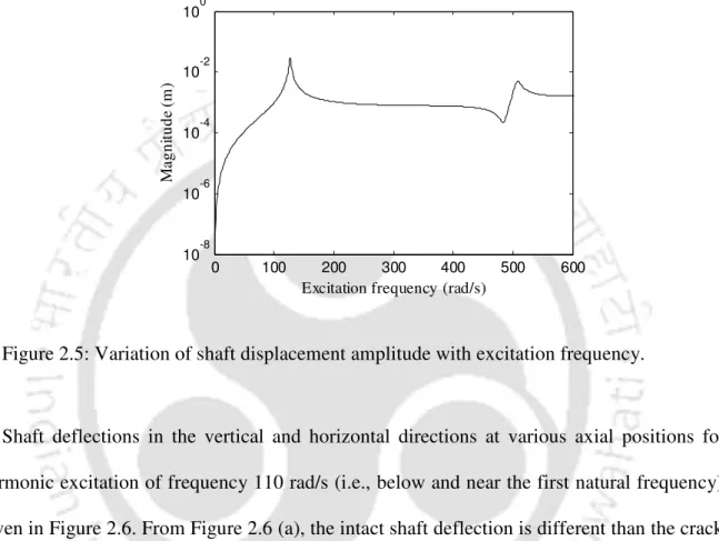
From standard eigenvalue analysis, the first two eigenfrequencies of the undamaged shaft were found to be 126.78 rad/s and 506.93 rad/s. In Figure 2.6 (a), the bending of the intact shaft is different from the bending of the cracked shaft in the vertical direction. The displacements in the vertical and horizontal planes are independent for the undamaged shaft, so the response of the undamaged shaft in the horizontal direction is zero (Figure 2.6 (b)).
Introduction
The MCDLA
There is no response in the horizontal plane to the vertical forcing of the intact shaft. Since there is no reaction in the horizontal direction due to the vertical forcing of the intact shaft, corresponding polynomial coefficients are therefore not defined. These coefficients give some degree of change in the vibration response with respect to excitation frequency at a specific location of the shaft.
Numerical Experiments of the MCDLA
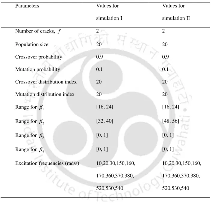
Simulation-I
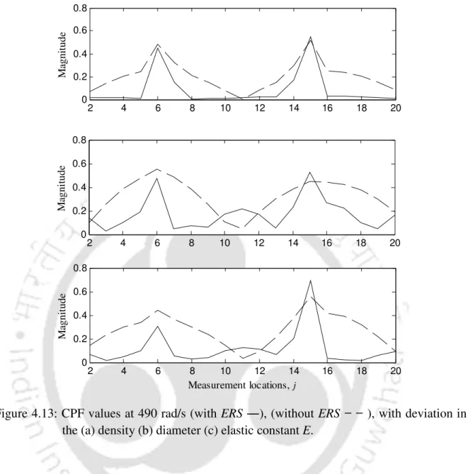
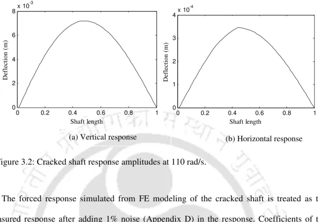
The forced response of the cracked shaft at the frequency ωi = 110 rad/s for different axial positions in the vertical and horizontal directions is shown in Figure 3.2. These two coefficients are used to obtain the normalized coefficients avIIi j in the vertical direction. Now the presence of cracks in the shaft can be seen from Figure 3.6 in the sense that peaks appear (inverted or upright) at the places of the cracks.
Simulation-II
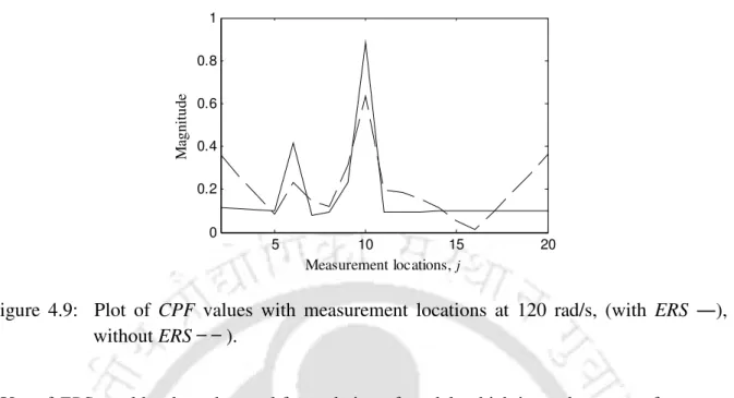
This therefore indicates the presence of two cracks in the shaft, one between locations x5 and x7, while the other between locations x9 and x11. This indicates the presence of two cracks in the shaft, one between locations x5 and x7, while the other between locations x13 and. The algorithm gives the number of cracks present in the shaft and their locations across the shaft.
Introduction
Introduction to Genetic Algorithm
Working Principles of Genetic Algorithms
- Binary Coding of the Strings
- Fitness Function
- The Selection Operator
- The Crossover Operator
- The Mutation Operator
- The Elitism Operator
- Termination Criterion
In the proportional selection, a string is selected for the matching pool with a probability proportional to the suitability of the string. The job of the crossover probability is to keep some strings in the matching pool unchanged after the crossover. In this way, some of the good strings from the mating pool are brought into the new generation unchanged.
The Multi-Objective Genetic Algorithm
Non-Dominated Sorting
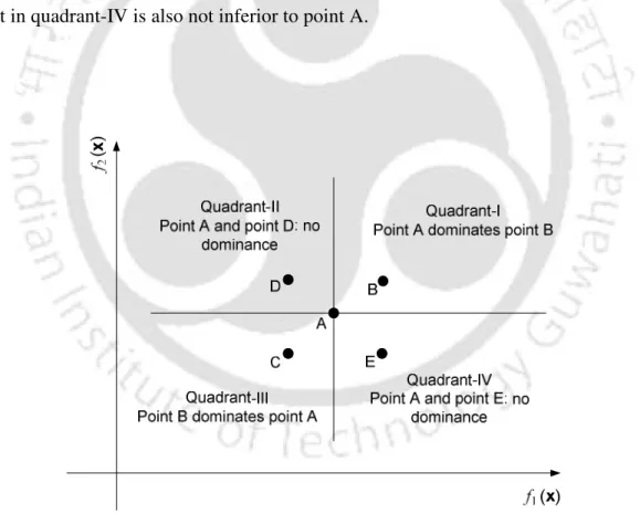
Since the optimization problem in Eq. 4.9) is a minimization problem, point A dominates all points in quadrant-I and all points in quadrant-III dominate point A. In non-dominant population sorting, those sets which are not dominated by any other set in the population are first identified. A new nondominated set of strings is then formed after temporarily neglecting the strings with rank 1.
Crowding Distance
Multi-Objective Optimization for Crack Parameters Estimation
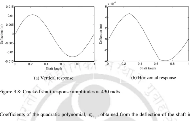
In fact, now combination III (crack depth ratio 0.73 at element number 51) results in a similar response to combination I. Also according to Figure 3.2, the response in the horizontal direction is much less due to the coupling effect than the response in the forcing direction, i.e. To give sufficient weight to the response in the horizontal direction, separate objective functions are constructed from this: one for the response in the vertical direction and one for the response in the horizontal direction.
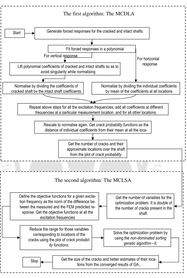
The MCLSA
To give a sufficient weight to the response in the horizontal direction, separate objective functions are made of it: one for the response in the vertical direction and one for the response in the horizontal direction. axis bending at frequency, ωi, and node , j, from. q in the vertical plane and. Similarly, that the deflection predicted by the cracked shaft model from. q in the vertical plane, and. Here, nc is the number of cracks present in the shaft, ne is the number of finite elements used to model the shaft, ds is the size of the crack, and R is the radius of the shaft.
Numerical Experiments for the MCLSA
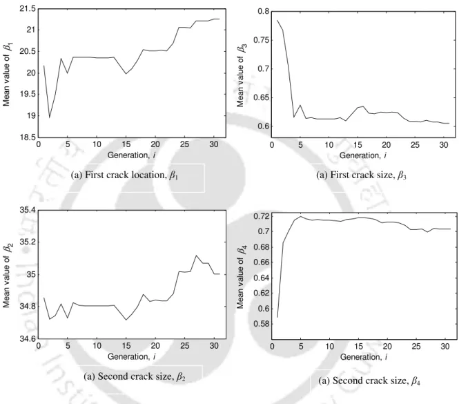
A flowchart of the above two-stage identification algorithm (the MCDLA and the MCLSA) is summarized in Figure 4.7. Narrow the range for the variables corresponding to the locations of the cracks using the crack probability plot. NSGA-II is used to solve the optimization problem that provides the dimensions and accurate locations of the cracks.
Normalization of the Quadratic Coefficients using “Equivalent Reduced Stiffness”88
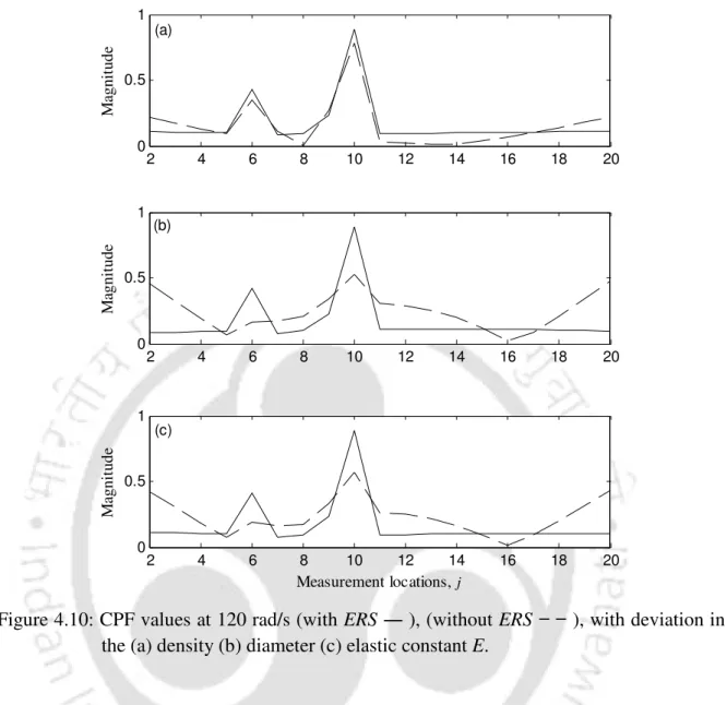
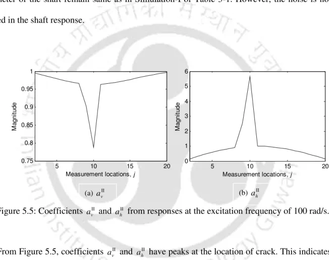
Measured responses of the cracked shaft are generated with 2% change (reduction) in values of the density, diameter and elastic constant E (not all simultaneously, but one at a time). Now the algorithm for simulation example II is tested for the case where the density, diameter and elastic constant of the cracked shaft and the intact shaft are not the same. Cracked shaft responses are generated with 2% change (reduction) in values of density, diameter and elastic constant.
Introduction
Identification of Open Cracks
Shaft Response with Rotated Open Crack
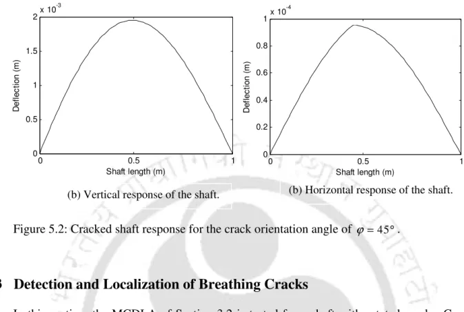
The flexibility matrix of the cracked element in the X'−Y'−Z' coordinate system is the same as Eqn. Therefore, the response of the shaft in the X'−Y'−Z' coordinate system can be generated for a forcing given by Eqn. Let the deflection of the shaft in the Y' direction be represented by qy' and the deflection of the shaft in the X' direction be represented by qx'.
Detection and Localization of Breathing Cracks
Estimation of the Crack Orientation Angle
These variations (i.e. peak size versus crack orientation angle) are plotted in Figure 5.6. For this it is proposed to obtain the coefficients avII and ahII at regular angular positions of the axis. Therefore, it is justified to take the shaft response at different angular positions of the shaft to obtain the crack orientation angle.
Identification of the Crack Size
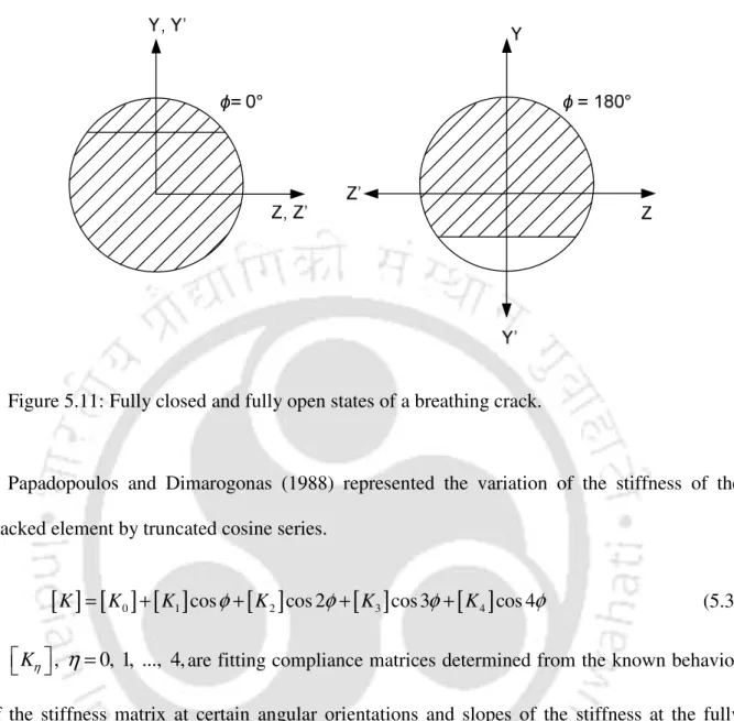
When cracks are entirely in the compression zone, the cracks will be completely closed and the stiffness of the shaft element containing the crack will be the same as that of the intact shaft. Also, when the shaft is partially open and partially closed, the effect of cracks on the dynamics of the shaft movement will be less than when the cracks are completely open. At part of the angular orientation, when the crack is open, the effect of the crack would be more on the dynamics of the shaft, which will help the condition monitoring system to find out crack parameters.
Identification of Breathing Cracks
- Shaft Responses for Breathing Cracks
- Detection and Localization of Breathing Cracks
- Estimation of Crack Orientation Angle of Breathing Cracks
- Identification of Crack Size
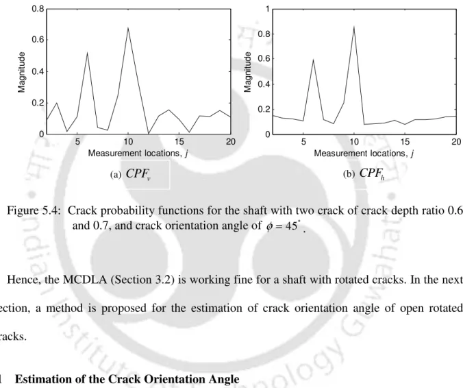
In the next section, an algorithm for estimating the crack orientation angle of respiratory cracks is presented. In this section, an algorithm for estimating the crack orientation angle of breathing cracks is presented. The crack depth ratio and crack orientation angle were taken as 0.7 and 0°, respectively.
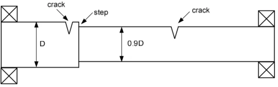
Detection and Localization of Cracks in a Stepped Shaft
The MCDLA is based on the detection of the slope discontinuity present in the elastic line of the shaft. In the above two examples, the crack orientation angles for the two cracks are taken as zero. For the second example (first crack near the measurement location 7 and the second near the measurement location 12 with step in the shaft near the measurement location 7) is given in Figure 5.26(b).
Introduction
Experimental Setup and Instrumentation
- Experimental Setup
- The Excitation Unit
- Signal Generator and Power Amplifier
- Force Transducer
- Proximity Transducers
- Laser Vibrometer
- Data Acquisition System
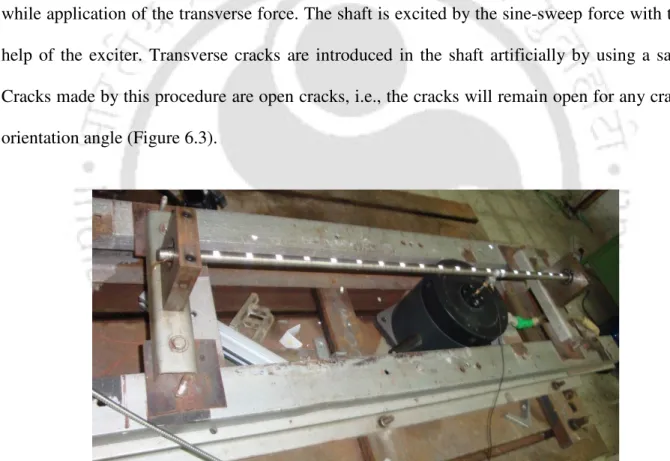
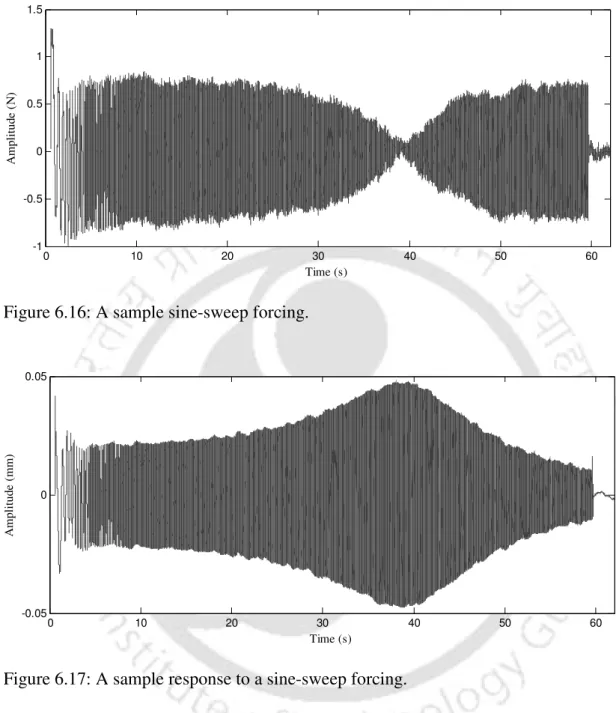
The cracks produced by this process are open cracks, meaning that the cracks will remain open for any angle of crack orientation (Figure 6.3). Sweep-sine (continuously changing the frequency of the signal) can be used for both sine and double sine signals. The following are the characteristics of the force transducer (B&K, model 2311-1) used in this experiment.
Stages for Conducting the Experiments
First, measurements were performed with the proximity sensor; However, after not getting satisfactory results with the proximity sensors, the rotation laser vibrometer was used. Procedure for conducting experiments using proximity sensors, along with required signal processing is discussed in the following sections.
Experimentation using Proximity Sensors
Procedure
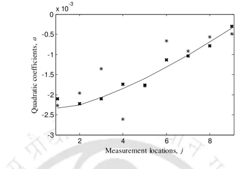
The CPF values for the I-Axis for the second set of measurements are given in Figure 6.24. The CPF values from the first set of measurements, for Axis-II with two slits, are shown in Figure 6.29. The CPF values (from the second measurement set) for Axis-II with two slits are shown in Figure 6.30.
Signal Processing of Measured Signals
Experimental Results
Experimentation using Laser Vibrometer
Procedure
The laser beam is sharp, so it can be focused on small points. However, there are some problems with focusing the beam over dot marks: (1) the dot mark is not visible due to glare in the beam, and (2) it is advised not to stare into the laser beam for long periods of time. In this way, correct focus is achieved by aligning the laser beam along the two marking lines.
Signal Processing of the Measured Signal
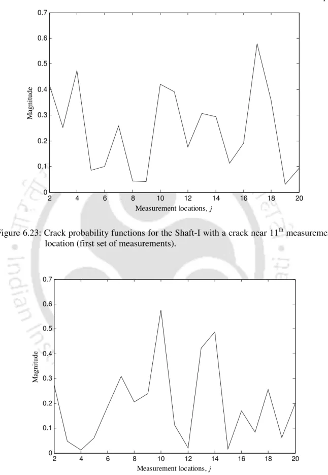
Now all force amplitudes are fitted to a degree 20 polynomial to further smooth the curve and is shown in Figure 6.18. Response amplitudes at several other measurement locations are shown in Figure 6.20. a) Force amplitude for the full measurement time. The axis deviation at a given frequency is obtained from the response per unit force at all these measuring locations.
Experimental Results
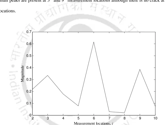
Figure 6.27 shows that there is no peak in the CPF values at either location, while in Figure 6.28 a single peak appears at the eleventh measurement location. For the shaft-II with two cracks, the algorithm detects the crack at the 13th measurement location (which is almost in the middle of the shaft) in both measurement sets. Good performance of the algorithm for the Shaft-II can be attributed to the larger size of the cracks.
Scheme for Better Estimation of the Quadratic Coefficients
The Scheme
In the next section, a scheme is presented to estimate the quadratic coefficients more accurately. In the following sections, the workings of the scheme are explained with numerical simulation examples.
Numerical Simulation of the Scheme
In simulation A, the noise is taken as 1% and the number of measurement locations is taken as 21. Now the number of measurement locations is reduced and thus the distance between two measurement locations is increased. Therefore, the algorithm identified the presence of crack when increasing the distance between two measurement locations.
Implementation of the Scheme to Actual Measurements
The crack probability functions for the second set of measurements on Shaft-I with a single crack near 6th measurement locations are given in Figure 6.37. CPFs obtained from the second set of measurements for the same condition (Shaft-II with single crack at 7th measurement location) are given in Figure 6.39. The crack probability functions obtained from the first and second set of measurements are presented in Figure 6.40 and Figure 6.41 respectively.
Conclusions
To further improve the experimental predictions, a scheme is proposed to better estimate the double derivative of shaft deflections. MCDLA is developed for the initial detection and localization of cracks present in the shaft. It is based on the detection of a break in the slope in the elastic line of the shaft.
Limitations and Applicability
Scopes for the Future Work
More analytical study would be necessary to understand (i) the stepwise variation of the coefficients (ii) the dependence of the angle 23° with the crack depth and the shaft diameter. The dimensionless expressions for the flexibility matrix []C (Figure 2.2) are given by Papadopoulos and Dimarogonas (1987).
Elemental Mass Matrices
The element stiffness matrix
Elemental Displacement Vector for Transverse Vibrations