Non-standard scalar field models of inflation and their reheating dynamics

For purposes of illustration, some figures in this assignment are taken from other sources and properly cited. We also discussed the origin of the plateau potential from supergravity and the general scalar tensor theory.

A brief review of standard cosmology

From the above equation, the evolution of the energy density can be written as the well-known continuity equation. If you go further back in time, when the age of the universe is about 380,000 years, it is.

Basics of Inflation

While the symmetries of the standard models predict almost equal amounts of matter and antimatter in our universe. We do not have a precise understanding of the state of the universe before inflation.

Figure 1.2 : Fluctuations in the Cosmic Microwave Background (CMB) [Image courtesy: ESA website]

Inflation: A period of exponential expansion

More on conditions for inflation: Slow roll parameters

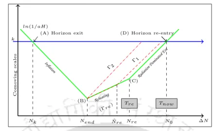
The scale of homogeneity, as observed in the CMB or large-scale structures, is quantified by the aforementioned inflation parameter N. The current size of the observed homogeneous universe can be well explained by the fact that this e-folding number is ∆N = 50 ~ 60.

Scalar field as the source of inflation

With this expression for energy density and pressure, we easily obtain the equation of state for the inflaton as,. The dynamics of the inflationary background phase is described by the following set of homogeneous equations for the inflaton and the scale factor derived from the action Eq.

The slow-roll conditions

Therefore, in this section our discussions will mainly focus on the basic methodology of how to derive inflation from inflaton. However, the stress-energy tensor associated with the inflaton turns out to be

Cosmological Perturbations

Metric perturbation
Matter Perturbations
Gauge invariant variable and power spectrum: scalar mode
Tensor Mode
Observations and constraints

It has been proven that this small density fluctuation is the cause of the observed temperature fluctuations in the CMB. In the cosmological context, the general form of the perfect energy momentum tensor takes the following form.

Figure 1.3 : The curvature perturbations R generated during inflation do not evolve once they exit the horizon.

Inflationary Models

Large field models

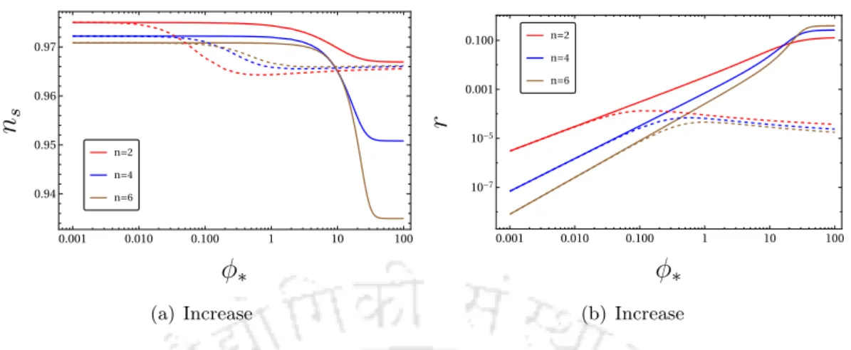
Once we have established the value of the model parameter, the spectral index and the scalar-to-tensor ratio can be predicted as .

Small field models

The amplitude of curvature disturbance takes the following from, PR= λ(φ2k−v2)4. 1.97) where the second and third approximations are made for small fieldφkvandφe∼(x−√. The small-field models that predict small values of scalar-to-tensor ratio are therefore favored by data.

Hybrid Inflation Models

The number of e-folds N from the start of inflation at φk to the end of inflationφe is expressed as. The figure shows that inflation in itself is not the end of the story.

Reheating after inflation: perturbative

Non-Perturbative Reheating or Pre-heating

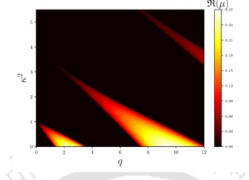
Depending on the values of the parameters (κ, q), this solution will grow exponentially when R(µκ,q)>0, which is identified as the particle production. Another important effect, which goes against the effectiveness of narrow resonance, is the decrease in inflaton amplitude with time.

Figure 1.10 : instability bands of Mathieu/Hill type equations. For parameters (q, κ) value within a instability band, the equation will show exponential growth.

Motivation of the thesis

Background Equations

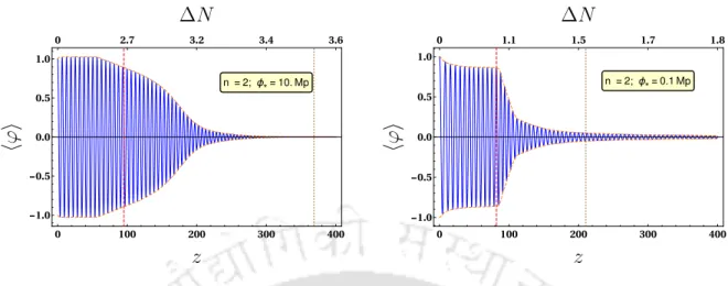
In this section we will study in detail the background dynamics using the above form of potentials. Let us also define a higher order slow spin parameter related to the third derivative of the potential for the spectral direction. Using the aforementioned boundary conditions for the inflaton we have solved for the homogeneous part of the inflatonφ(t) and the scale factor (t).

As we mentioned, the inflation ends when = 1, and one can use Eq.(5.69) to find the value of the inflaton at the beginning of the inflation. It is clear that the above analytical expressions for the inflationary observables derived in Eq.(2.15) are valid for subplanck values of the scale φ∗. In Table2.1 we have given some sample values of all the cosmologically relevant quantities for different values of the model parameters.

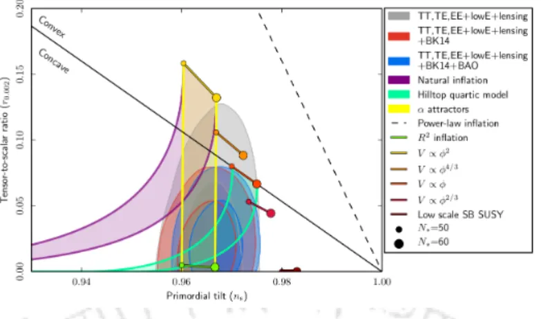
Figure 2.1 : The n s -r plot of the model on the marginalized joint 68% and 95% CL regions at k = 0.002M pc −1 from Planck alone and in combination with BK14 or BK14 plus BAO data[19].

End of inflation and general equation of state

Therefore, it is clear that the conventional study of the preheating and reheating phase is applicable to this model. In this section, we will discuss the CMB constraint on the reheating phase, while the preheating and excited reheating for the model will be studied in the following sections. In the next section, we describe a possible realization of the potential of our model from the general scalar-tensor theory, and in the next section we will also provide a realization of our model in N = 1 supergravity.

Towards derivation of V min from non-minimal scalar-tensor theory

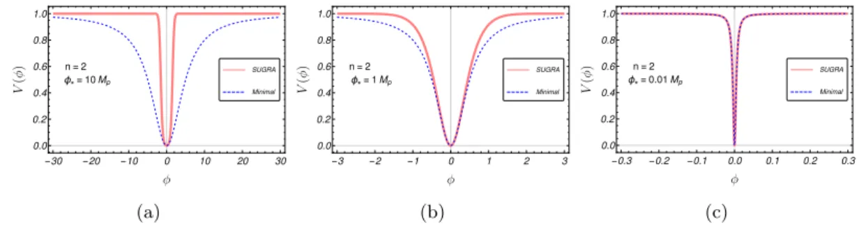
It can be seen that the potential of the model around the minimum is given by their power-law behavior. Supergravity realization of our model potential Now, we choose the following non-minimal coupling function [62,75], forΩ2(φ),.

Supergravity realization of our model potential

The power-law plateau potential form Supergravity

As a first simplification, we will assume that the functional form of the holomorphic functions F1 and F2 are the same, that is, F1≡F2. The d. The charge of the fields Φ1 and Φ2 (whose modulus will be identified as the inflaton) must disappear. It is clear that the supergravity potential Vsugra and our minimum plateau potential Vmin are identical for the sub-Planckian values of the scale φ∗.

Figure 2.3 : Comparison of the shape of the two potentials for three different values the scale φ ∗

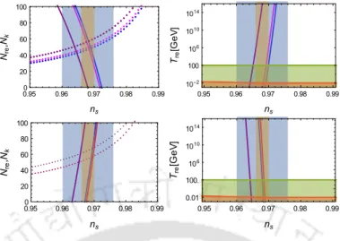
Model independent constraints from reheating predictions

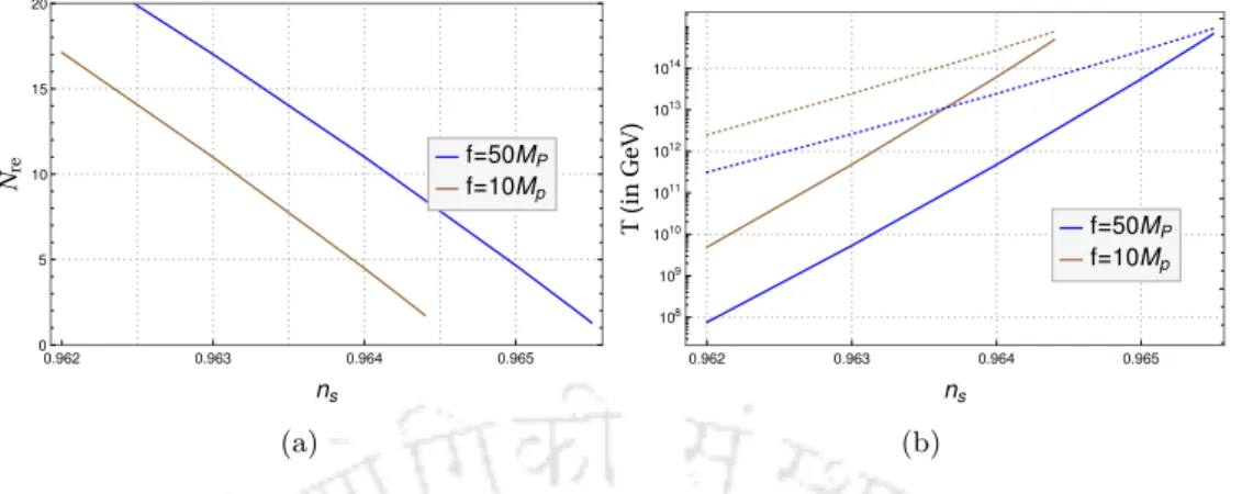
Where,Nre1, Nre2 develop a number during the first and second phase of the warm-up phase with the equation of statewre1, w2re respectively. Therefore, the equilibrium temperature after the end of the heating phase, Tre, is related to the temperature (T0, Tν0) of the CMB photon and neutrino background on the current day, respectively, as follows. With increasing value of the equation of state, the e-folding number during reheating Nre decreases for a fixed value of the reheating temperature.

Figure 2.5 : variation of the spectral index (n s ) and scalar-to-tensor ratio with the scale φ ∗ for the two potentials.

Summary and Conclusion

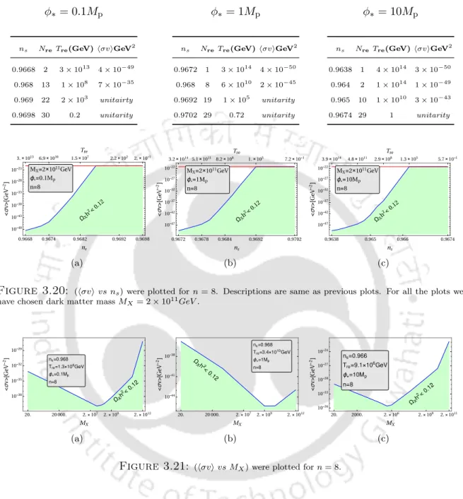
In the present epoch, apart from the cosmological constant, dark matter and CMB are the two main components of our universe. Dark matter is believed to play one of the important roles in the aforementioned processes of structure formation. From the background evolution, we know that our universe is dominated by 23% dark matter from the total energy budget of the universe.

Inflationary observables and their connection with CMB

The tensor-scalar relation associated with the inflationary energy scale has its own signature in the polarization modeB of the CMB, which has not yet been observed. All these quantities are defined for a certain cosmological scale, which is the CMB spin scale, k/a0 = 0.05Mpc−1. These quantities will be described in the appropriate places, but before that, in the next section we will review the Boltzmann equation for the three different components of energy, namely the inflaton, radiation, and dark matter.

Dark Matter during reheating

Basic equations

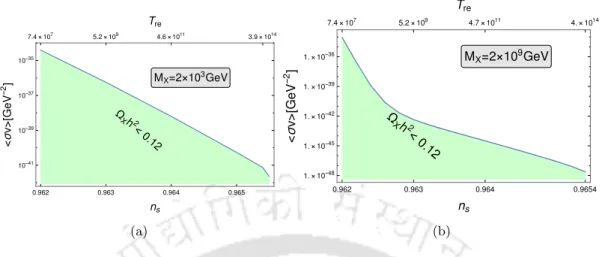
For our further discussions, it is important to know the behavior of the dark matter abundance in terms of the reheating parameters (Tre, MX, hσvi). Analytical expressions for the dark matter abundance for different MX dark matter masses can be calculated following references [106] (see also [107,108] for an alternative derivation). Since we have considered the generic equation of state parameter for the inflaton, we are interested in a generalized expression for the dark matter abundance for any wφ.

Constraints from CMB: dark matter phenomenology

Connecting CMB and reheating via inflation
Methodology: CMB to dark matter via reheating
Chaotic inflation: General results
Natural inflation
Alpha attractor
Minimal Plateau model

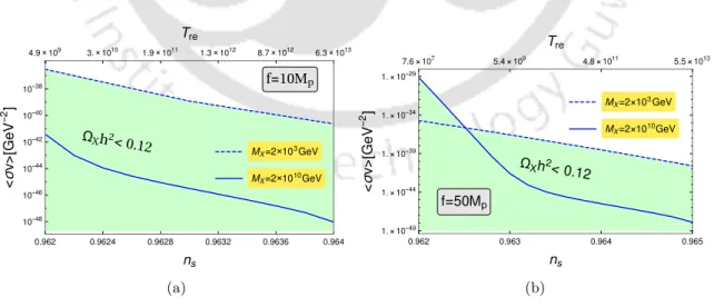
Due to the limited abundance of dark matter in the present universe, we can establish a direct connection between CMB anisotropy and dark matter phenomenology. Here we consider the (a)109GeV and (b)103GeV dark matter masses for the chaotic cm2φ2 model. However, we will consider the production of dark matter through the freezing mechanism in this work.

Figure 3.1 : The comoving scales connect the inflationary phase with the CMB. The solution of Boltzmann equations for inflaton decay will connect the end of inflation denoted by the point B and beginning of radiation domination denoted by the point C, and

Summary and outlook

An important assumption in our analysis that needs further investigation is the assumption of a perturbative breakup of the inflaton during reheating. Finally, let us elaborate on one more issue, which we already mentioned in the last point of table 3.4. The problem is related to the relationship between the CMB anisotropy and the primordial anisotropy originating from the quantum fluctuation of the inflaton field.

Figure 3.20 : (hσvi vs n s ) were plotted for n = 8. Descriptions are same as previous plots

A Brief Introduction to the Minimal Inflation Model

A Brief Introduction to the Minimal Inflation Model Value range of the coupling parameter that will set the value of the above perturbative.

Preheating: Parametric resonance

The Model and equations

The energy density of the universe immediately after the inflation is in the form of the homogeneous inflation field. This energy begins to decay into fluctuations in the buoyancy and other fields at the onset of preheating. However, the rapid energy drain due to exponential particle production affects the dynamics of the blowing field.

Parametric resonance: Instability chart

Therefore, we will naturally need a higher value of the coupling constant to obtain resonance. They depend on time via the scale factor and the time-dependent amplitude Φ(t) of the inflation fluctuation. Nevertheless, we can include the effect of expansion in the instability analysis by taking into account the fact that the amplitude of the inflaton oscillation will decay as Φ∝a−6/(n+2).

Preheating: Lattice Simulation

The back-reaction and the emergence of non-linearity: Generalities
Equation of state
Occupation Numbers
Perturbative reheating and constraints from CMB

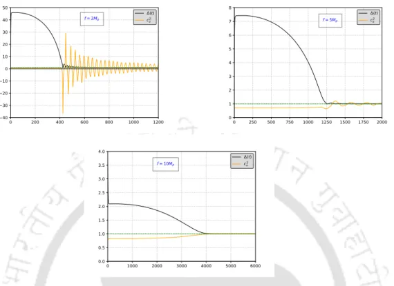
In fig (4.4), the two left panels describe the evolution of each individual energy component in the inflaton and the reheating field with respect to toz. The equation of state is one of the most important parameters to study during preheating. The solid blue lines are the instantaneous value of the equation of state, while the red dashed line is the average value over a period of inflaton oscillation.

Figure 4.3 : Evolution of volume averaged comoving inflation amplitude ϕ = (a/a i ) 3/2 (φ/φ 0 ) for the model potential n = 2 for φ ∗ = 10M p and 0.1M p

Conclusion and Outlook

Similar observations have been made in recent works[165] examining the self-resonance of inflation for similar plateau-type inflation models. Clearly, preheating itself is not the full story of heating dynamics. If both interactions are present, we will have several interesting behaviors of the system [177, 178].

The most General Single-Field Inflation

Potential-driven G-inflation

In the case of kinetically driven G inflation, the shift symmetry of the original Lagrangian remains intact. The shift symmetry does not allow any potential term. rewarming dynamics, one has to introduce a new mechanism. Within the Galilean framework, we can consider potential driven slow-roll G inflation, where the potential term clearly breaks the shift symmetry of the Galilean model.

Perturbations in Generalized G-inflation

Now we write the action for the scalar perturbations by setting hij = 0, the second-order action is given by Potential-driven G-inflation with a shift-symmetric potential Finally, the scalar spectral index(s) and tensor-to-scalar ratio(s) are given by.

Potential driven G-inflation with a shift symmetric potential

G-axion

For our later convenience, we note the following relationship between the KGB function and the slow roll parameter. Which tells us that although the higher-derivative term dominates the dynamics of slow-roll inflation, the standard part of the Lagrangian remains much larger than the Galileon part during inflation (1), and they both became comparable only after the end of inflation (= 1). Using Eq.(5.62), the condition that the KGB term dominates the usual slow-roll term can be monitored by defining a parameter.

As highlighted in the introduction, the usual canonical axion inflation scenario is strictly constrained with respect to the PLANCK observation. We will see that for a wide range of parameter spaces, higher derivative terms will play a major role in the G-axion inflation.

Number of e-folds and modified Lyth bound

We are therefore able to compare the Lyth limit between G-action inflation and ordinary canonical slow-roll inflation, which can be written in a model-independent manner as ∆φ-slow-roll ∼ Eg. Now since we have freedom in choosingf, the modified Lyth connection can become very small. In the next section, we will consider some simple phenomenological forms of the KGB functions keeping the constant Lagrangian displacement symmetry intact and construct the PLANCK-compliant super- and sub-Planckain inflation models.

Simple choices of M (φ) and determination of cosmological parameters

Evolution of the scalar field: sub-Planckian (f, s)

Although these instabilities can be avoided for larger values of the action decay constant, we are mainly interested in subplank values down. In our numerical calculation, it was found that the scalar field does show singularity or oscillatory behavior, depending on the values of the above parameters. It was found that the minimum value of the coefficient tends to zero with decreasing f.

Figure 5.3 : The evolution of (∆(t), c 2 s ) with time for three different values of the axion decay constant for M(φ) = Sin(φ/f) when A = 92

Non-oscillating axion: Instant preheating

Conventional Shift Symmetry Breaking Coupling

Let us start by considering the interaction Lagrangian as from the original work of Felder-Kofman-Linde. The production of the χ initiates as mχ begins to change non-adiabatically after the end of inflation. And with this value of coupling constant, we can easily check that the production of the χ particle is indeed instantaneous.

Shift Symmetric Coupling

Even though the particle production at the time of the first zero crossing of the inflaton seems inefficient, for the sake of completeness let us restrict the possible value of h for the operation of the instantaneous preheating mechanism. For instantaneous preheating to work, it must be greater than the expansion rate of the universe at the time of preheating. As we concluded from our analysis, the instantaneous preheating mechanism proves to be inefficient for the conventional shear symmetry breaking coupling discussed above.

Conclusions