Siddhartha Pratim Chakrabarty, Associate Professor, Department of Mathematics, Indian Institute of Technology Guwahati for the award of the degree of Doctor of Philosophy and this work has not been submitted elsewhere for the degree. The thesis work entitled “Numerical Methods for Passport Option Pricing” by Ankur Kanaujiya, a student in the Department of Mathematics, Indian Institute of Technology Guwahati, is certified as having been completed for the award of the degree of Doctor of Philosophy. under my supervision and this work has not been submitted elsewhere for a degree.
Brief background
Solving the HJB equation, which is a backward partial differential equation (PDE), provides the price of the passport option. The passport option pricing problem using a jump-diffusion model (which addresses some of the shortcomings of GBM) for the underlying traded security was.
The passport option
Kampen [21] considered a multivariate passport option to determine the optimal strategy, which turned out to depend on correlations between returns and those of the Greeks. The interested reader can refer to [5, 22] for a comprehensive review of the passport option in both discrete (binomial) and continuous time settings, noting that the optimal passport option strategy is identical for both models and that the binomial model converges to the continuous time model.
Outline of the thesis
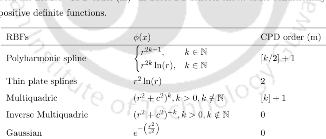
The shape function used in the case of PIM is the Kronecker delta function, which makes it suitable for setting the boundary condition [31]. Unfortunately, a systematic protocol for determining the shape parameter values was not found in the literature.
Numerical implementation for the symmetric case
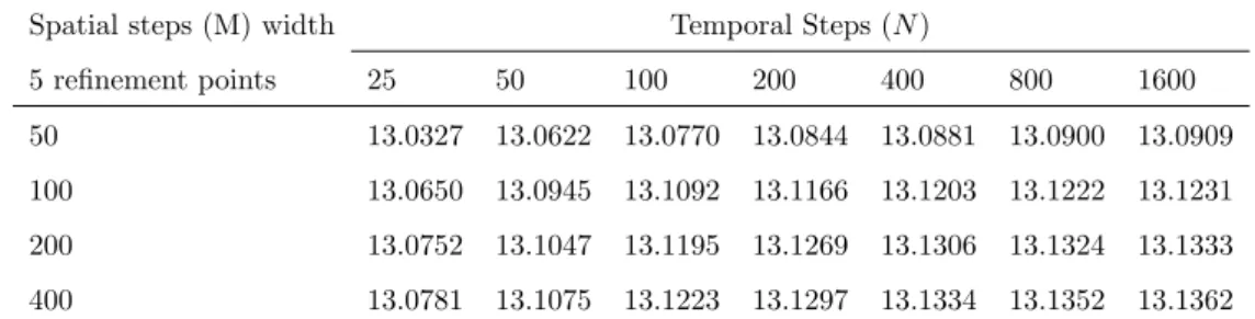
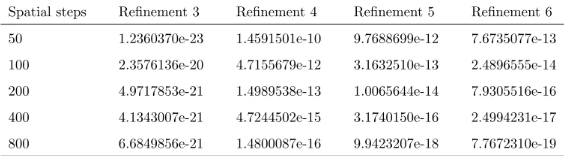
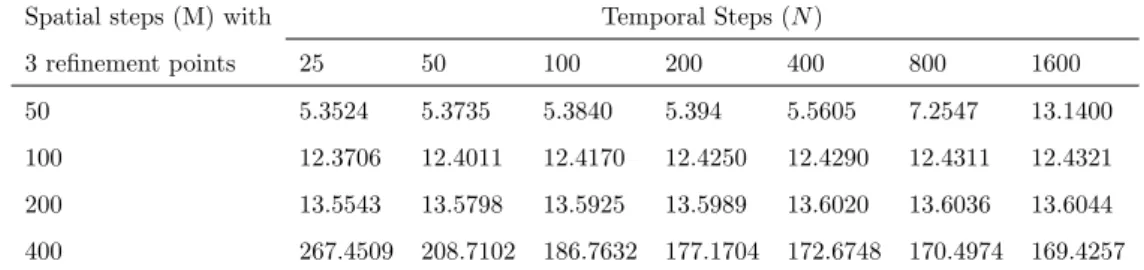
In Table 2.3, the results for the European passport option are shown with 4 refinement points for several different sets of the number of spatial and temporal grid points. Thercond(G) for 3,4,5 and 6 refinement points in case of several spatial steps are presented in table 2.6.
Numerical implementation for the non-symmetric case
The diagram (2.3.5) on the interior points together with the boundary conditions can be written in the compact matrix form as. We now present the numerical results for the RBPI method, detailed in the equation for the non-symmetric case. The calculation was performed for different mesh sizes and for refinement points, as was done in the caser=γ.
It can be seen that the values tabulated in Table 2.7 are very close to those reported in [3] and [4]. Finally, the reciprocal condition number, rcond(G) for all four refinements with N = 50 are shown in Table 2.9. Based on the second(G) reported in Table 2.9, we note that in the case of refinements 3,5 and 6, the interpolation matrix Gis is either singular or ill-conditioned.
Conclusion
In this chapter, we investigate the numerical approach for the symmetric case and the non-symmetric case for the European-type fitting option using three time levels. This particular concern will be addressed in this chapter by using a three-time-level finite-difference scheme, where one can use larger time steps (i.e., smaller number of time points) while ensuring the accuracy of the solution to the valuation PDE along with the evaluation of the Greeks, namely Delta, Gamma and Theta. Remember that the dispersion time of the pass option pricing PDE (both symmetric and non-symmetric case) is non-smooth.
Accordingly, we will use scheme 9 (as mentioned above), which is akin to a three-level version of the Crank-Nicholson scheme. Note that both the spatial and temporal accuracy of the three-time level scheme are second order. Since we now have three time levels, information at two prior time levels is needed to numerically evaluate the value at the current time level.

Three time level scheme for the non-symmetric case
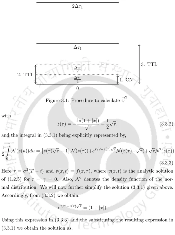
The procedure for calculating →v2 for both the symmetric and non-symmetric case is illustrated in Figure 3.1. Once →v2 is determined, values from →v3 onwards are determined using the three time level scheme. Finally, the optimal retention strategy given in (1.2.4) is discretized as follows. 3.2.6) To discretize the Neumann boundary condition (2.2.2), we used the second-order central difference approximation for vx.
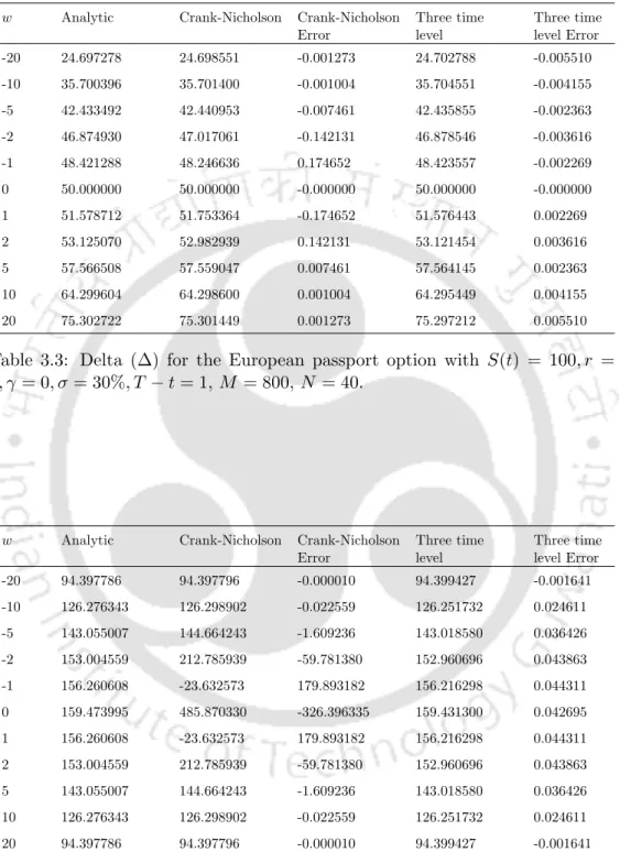
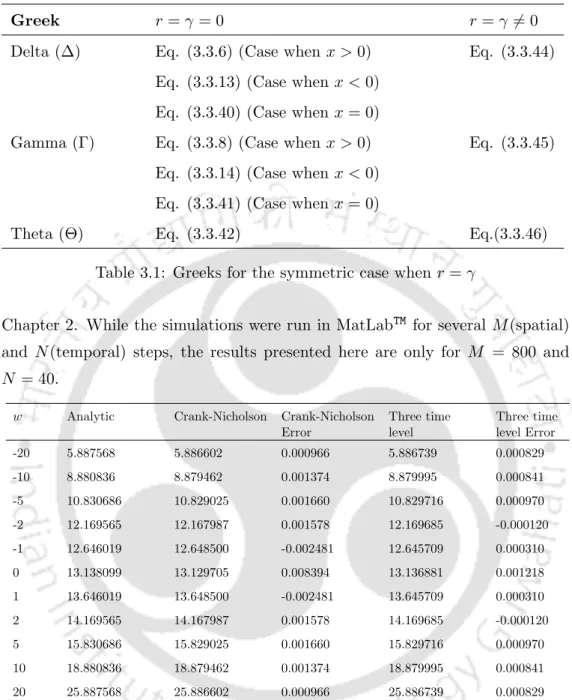
Valuation of Greeks: Delta, Gamma and Theta
Numerical results
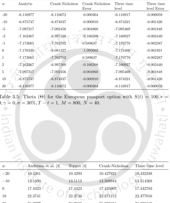
Further, near=0, it was observed to be 10−3 with a somewhat smaller error in the case of the three time level scheme. The error plot for the Crank-Nicholson scheme and the three-time-level scheme are shown in Figure 3.2 and Figure 3.3, respectively. This advantage is more clearly seen when we analyze Table 3.4 for the values of Γ forw∈[−5,5] with the error of the three-time level scheme being of the order of 10−2, but the error goes up to 103 using the Crank-Nicholson scheme .
Finally, for Θ values (Table 3.5) it is observed that in the range w∈[−2,2] the order is 10−3 using three time level scheme as opposed to the order ranging from 10−1 to 101 with Crank-Nicholson scheme. The tabulated results for the option price using the Crank-Nicholson scheme and three time level schemes are given in Table 3.6. We also present the values of Greeks for this (non-symmetric) case using the Crank-Nicholson scheme and three-time level scheme in Table 3.7 and Table 3.8.
Conclusion
Crank-Nicholson scheme
Using the above notation, (4.1.1) can now be written as sequence of linear complementarity problem as follows.
Three time level scheme
The discretized version of (4.0.2) using a finite difference scheme at three time levels [35–37] (as discussed in Chapter 3) can be written as,. However, for reasons already justified in Chapter 3, we will use the Crank-Nicholson when estimating the value →v2 using →v1, as discussed in Figure 3.1. The discretized pricing problem will now be solved via the outlined scheme, using the Brennan-Schwartz algorithm [41, 42] and the PSOR method [40, 43].
Therefore, algorithm (2) and algorithm (4) are used to solve the linear complementarity problem (4.1.3) using the Brennan-Schwartz algorithm and the PSOR method, respectively. The Brennan-Schwartz algorithm is used to solve the matrix form of the linear complementarity problem arising from the implicit discretization of the linear complementarity problem. Analogously, algorithm (3) and algorithm (5) are used to solve the linear complementarity problem (4.1.6) using the Brennan-Schwartz algorithm and the PSOR method, respectively.
Numerical results
Conclusion
The interior points
To determine these coefficients, Taylor series expansion for the terms (vx)mj+1 and (vx)mj−1 about the point (xj, tm) is carried out as follows. 5.1.3) Similarly, the Taylor series expansion for the terms vj+1m and vjm−1 around the point (xj, tm) is given by. To determine these coecients, Taylor series expansion for the terms (vxx)mj+1 and (vxx)mj−1 around the point (xj, tm) is performed as follows.
The boundary points
The following compact schemes are used to derive a fourth-order approximation to (vx)mM The following compact schemes are used to derive a fourth-order approximation to (vxx)mM−1,.
Matrix form
The discretization of u∗ in (1.2.4) using the HOC schemes is. 5.1.38) Note that the compact stencil was used only in the spatial direction, using the Crank-Nicholson scheme for temporal discretization. Accordingly, the HOC scheme would mean a HOC scheme in space and a Crank-Nicholson scheme in time.
Grid stretching
5.1.38) Note that the compact stencil was used only in the spatial direction, using the Crank-Nicholson scheme for temporal discretization. The temporal semi-discretization of (5.2.2) using the CNIM is as follows. 5.2.13) The fourth order approximation of Vy and Vyy (similar to that of vx and vxx) is as follows. The pricing for the US Passport option is exercised through the following outcome, taking into account that the US option can be exercised on or before the expiration date.
In order to determine the value of the US passport option numerically, the following early exercise condition.
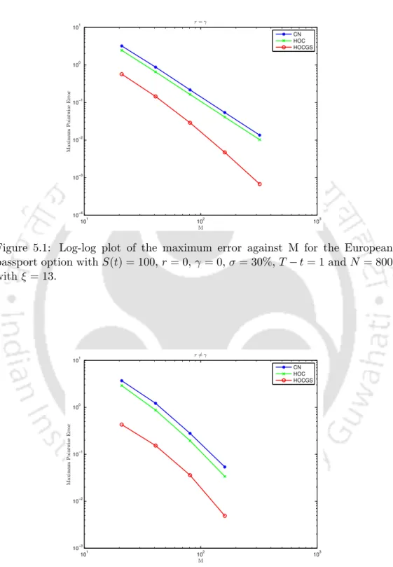
Numerical results
Apparently, while marginal maximum error reduction was seen for HOC scheme, significant reduction occurred when HOCGS scheme was used. Consequently, the maximum error and convergence rate are calculated using the double-mesh principle [51]. The maximum error and the rate of convergence are determined by the double mesh differences.
Further, the log-log plot of the maximum error as given by (5.3.1) against M (for the European option), are shown in Figure 5.2. Finally, the maximum error and convergence rate for this case using three schemes are given in Table 5.4 and Table 5.8, respectively. Also, the maximum error and the rate of convergence for several grid alignment parameters ξ and M are shown in Table 5.5 and.
Conclusion
The radial basis function approach was used to determine the price of the European passport option for both the symmetric and non-symmetric cases, with grid refinement used near the zero accumulated profit to improve the accuracy. Furthermore, improvement in the numerical option price and the Greeks was achieved using a three time level scheme for larger time steps for both cases. The three-time level scheme was then applied to price the US passport option with the corresponding discretized system solved using the Brennan-Schwartz algorithm and the PSOR method.
Finally, higher-order compact schemes are used to obtain the price of both the European and American passports with greater accuracy. TTL Spurious oscillations free and works well for the Greeks in case of larger time steps without loss of accuracy. HOC Better accuracy up to third order Unable to achieve fourth order accuracy and difficult to handle the uneven coefficients.
Future work
Chakrabarty, European passport option prices with radial basis function, International Journal of Applied and Computational Mathematics, vol.3, No. Kadalbajoo, A numerical study of Asian options with radial basis function based finite difference method, Engineering Analysis with Boundary Elements, vol. Morton, Differentiation method for the initial value problem, Interscience Tracts in Pure and Applied Mathematics, 1967.
Smith, Numerical solution of partial differential equations: finite difference methods, Oxford Applied Mathematics and Computing Science Series, 1985. Niu. , vol. Bhuruth, Numerical option pricing using compact higher order finite difference schemes, Journal of Computational and Applied Mathematics, vol.