It is noted that the methods presented in this part of the thesis for obtaining the first order potentials, and thus the reflection and transmission coefficients, greatly reduce the workload. These methods lead to a computationally more manageable form of the solutions for the scattered field.
Preamble
In this case, if it is assumed that the amplitude of the wave is small compared to the wavelength, then the theory is called linearized theory of water waves. The second class of problems, which are examined in the remainder of this thesis, .
Brief history and motivation of the present work
The mild slope approximation was used to reduce the governing boundary value problem to one involving a form of the Helmholtz equation where the coefficients depended on the topography. In such a two-layer fluid region, for a given frequency, time-harmonic gravity waves of two different modes propagate at each of the free surface and the interface.
Relevant basic equations in the linear theory of water waves
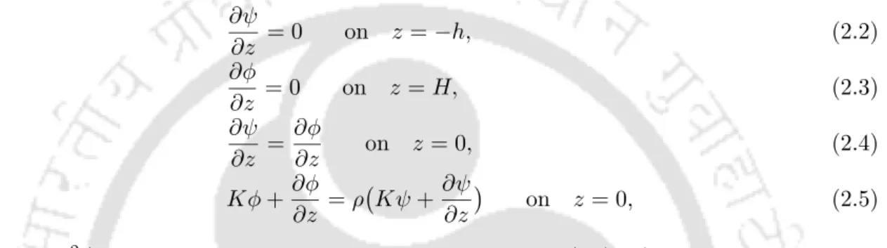
The condition (1.8) also gives the continuity condition of the normal component of the speed over the common interface. However, if the bottom fluid has a uniform finite depth H below the mean interface, the condition (1.15) is replaced by .
Outline of the thesis
In Chapter 7 we solve the reduced boundary value problem for first-order correction of the potentials for the oblique incidence case. The solutions of the boundary value problem for the first order corrections are obtained using the same techniques as applied in Chapter 6.
Mathematical formulation of the problem
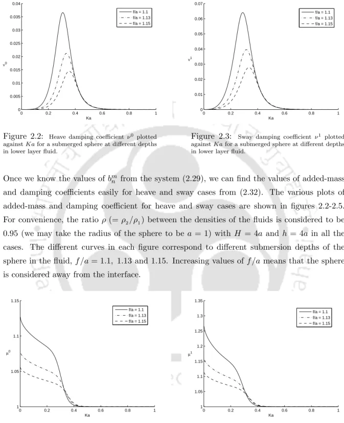
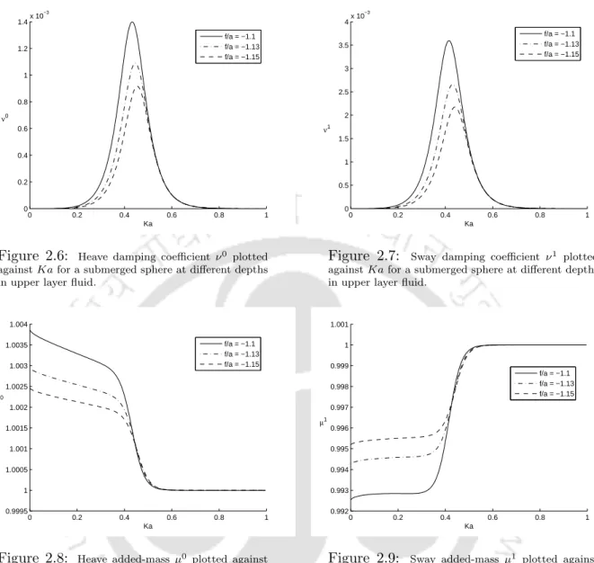
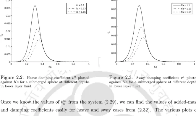
The corresponding problems of oscillation and oscillation radiation, either in the lower or upper layer, are solved by Thorn's multipole expansion method [73]; i.e. the coefficient of added mass and damping are evaluated for both cases. Numerical estimates for damping coefficients, added mass coefficients and exciting forces for both motions are calculated and plotted.
The radiation problem for a submerged sphere
Sphere in the lower layer
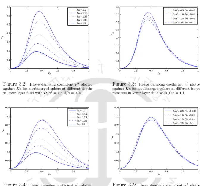
The solutions of the radiation problems for heave and sway are indicated by φ0 and φ1 respectively. The different curves in each figure correspond to different immersion depths of the sphere in the liquid, f/a and 1.15.
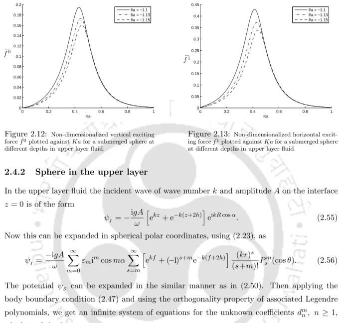
Sphere in the upper layer
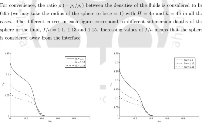
Figures 2.4 and 2.5, respectively, show the added mass coefficients for different depths of immersion for the heave and swing case. The different curves in each figure are studied for different depths of immersion of the sphere in the liquid, f /a and.
The scattering problem for a submerged sphere
Sphere in the lower layer
The same explanation, as given in Section 2.3.1, is valid for the convergence of the method. In each figure, the different curves correspond to different immersion depths of the sphere in the lower liquid, f /a and 1.15.
Sphere in the upper layer
Conclusion
The corresponding swing and swing radiation problems, either in the lower or upper layer, are solved by Thorne's multipole expansion method; that is, the added mass and damping coefficients are evaluated for both the cases. The numerical estimates for the damping coefficients and added mass coefficients for both motions are evaluated and plotted.
Mathematical formulation of the problem
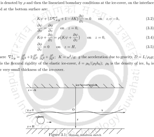
We solve the radiation problem for a submerged sphere placed in one of the layers of a two-layer liquid. L is the bending stiffness of the elastic ice cover, δ =ρ0/(ρ2h0); ρ0 is the density of ice, h0 is the very small thickness of the ice cover.
Solution by multipoles
Sphere submerged in the lower layer
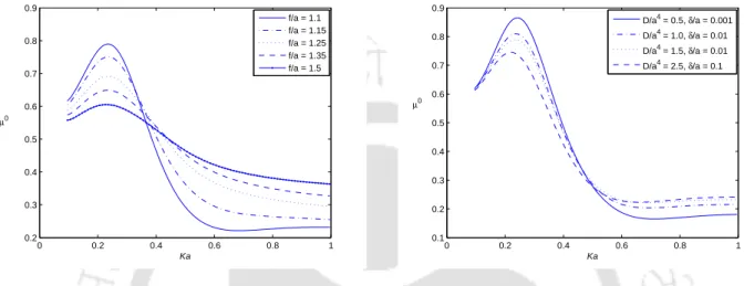
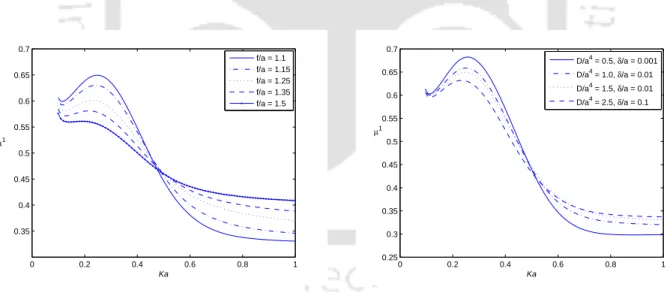
The solutions of the radiation problems in the case of lifting and swaying are denoted by φ0 and φ1, respectively. Figures 3.6 and 3.8, respectively, show the added mass coefficients for different depths of immersion for the heave and swing case.
Sphere submerged in the upper layer
Figures 3.3 and 3.5 show the damping coefficients for heave and sway cases respectively, whereas figures 3.7 and 3.9 show the added mass for the heave and sway cases. Figures 3.14 and 3.16, respectively, show the added mass coefficients for different immersion depths for heave and sway cases.
Conclusion
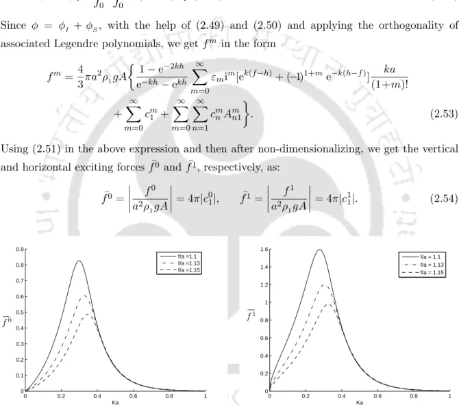
The reflection and transmission coefficients are subsequently evaluated approximately up to the first order of ε in the form of integrals involving the shape function which describes the small waveform. For the case of a patch of sinusoidal ripple bed when the ripple wavenumber is approx. twice the wavenumber of the incident interfacial wavefield, the first-order reflection coefficient is found to increase with wavenumber.
Mathematical formulation
The origin O is considered at the undisturbed interface between the upper and lower fluids, andy = 0 is the mean position of the layer interface. Due to this apparent mode of waves appearing in the liquid region, part of the interfacial shock wave is blocked and leads to a standing wave pattern over the bottom irregularities by the time the incident wave is dissipated by the bottom wave.
Perturbation technique
Reflection and transmission coefficients
Solution by Fourier transform technique
Splitting of boundary value problem
Fourier transform technique
Since ∆(ξ) has a non-zero zero at ξ =kon the positive real axis, the above integral in both cases contains a pole at ξ =k. Therefore, we indent the path for each integral in both cases under the pole at ξ =k.
Reflection and transmission coefficients
Special forms of bottom surfaces
Example-I
Although the theory falls apart when β = 1, that is, when l = 2k, a large amount of reflection of the incident wave energy will be generated by this special shape of bed surface near the singularity at β = 1. In practice, if the reflection wave is non-zero, there must be a progressive attenuation of the incident interfacial waves over the region L1 ≤ x ≤ L2.
Example-II
Therefore, under this condition, we can find the limiting value of the reflection coefficient R1 of (4.79) as . 4.81) As observed in Example-1, again R1 is a constant multiple of (m+n)/2, the total number of ripples in the plane of the corrugation. Although the theory does not work when either l1 = 2k or l2 = 2k, a large amount of reflection of the incident wave energy will be generated by this special bed surface shape near the singularities atl1 = 2k or l2 = 2k.
Numerical results
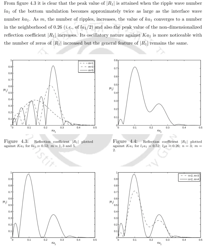
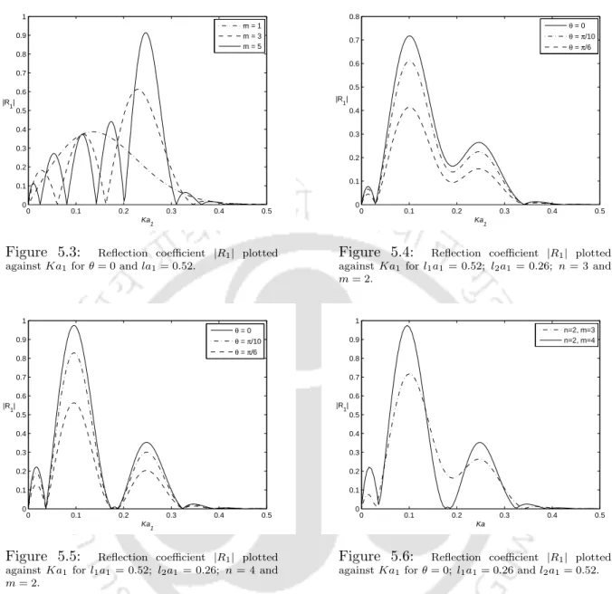
From figure 4.3 it is clear that the peak value for |R1| is achieved when the wavenumber la1 of the bottom wave becomes approximately twice as large as the interface wavenumber ka1. As m, the number of waves, increases, the value of ka1 converges to a number near 0.26 (ie, ofla1/2) and also the peak value of the non-dimensionalized reflection coefficient|R1|increases.
Conclusion
For this we consider the numerical calculations, calculated from (4.79), for the non-dimensionalized first-order reflection coefficient |R1|, due to an incident interface wave of wavenumber k, with two different ripple wavenumbers l1 and l2, respectively , with m and n number of ripple wavelengths in the dot of the bottom. Therefore, we observe from figure 4.5 that |R1| has two peak values that are reached when the ripple wavenumber1a1 andl2a1 of the lower corrugation becomes approximately twice the interface wavenumberka1.
Mathematical formulation of the problem
The work presented in this chapter deals with the scattering problem of Chapter 4, but here we consider a series of progressive (internal) waves propagating from negative infinity obliquely incident on the channel bed with small undulations. If it is assumed that for small bottom undulation ε is very small and the second order terms are neglected, here the boundary condition ∂φ/∂n = 0 on the lower surface y =H+εc(x) can be expressed in the same appropriate form ( 4.10 ).
Perturbation technique
Solution by Green’s function technique
Introduction of Green’s functions
Again, there will be no contribution to the integral from the line y=−h due to the same boundary condition that ψ1 and G2 satisfy there. Similarly, to calculate ψ1(ξ, η) when the source term (ξ, η), −h < η <0, is immersed in the upper layer fluid, we use the same procedure as followed earlier for the case of the lower layer fluid layer.
Reflection and transmission coefficients
Special forms of bottom surfaces
Example-I
Furthermore, when the bed wavenumber is twice the component of the interface wavenumber along the x-axis, that is, 2µ/l= 1, the theory indicates the possibility of a resonant interaction between the bed and the interface. Thus, the reflection coefficient R1, in this case, becomes a constant multiple of m, the number of ripples in the chip.
Example-II
Although the theory fails when β = 1, i.e. 2µ=l, a large amount of reflection of the incident wave energy will be generated by this special shape of bed surface near the singularity atβ = 1. The observations made in Section 4.6.1 about the violation in the conservation of energy in resolving the potentials for the normal incidence also applies to the oblique incidence.
Numerical results
Figure 5.3 shows that the highest value is |R1| reached when the wavenumber la1 of the bottom wave becomes approximately twice the wavenumber of the interface µa1. As m, the wavenumber, increases, the value of µa1 converges to a number in the vicinity of 0.26, i.e. for la1/2, where |R1| reaches its maximum, and the upper value of the non-dimensionalized reflection coefficient|R1| also increases.
Conclusion
Another key result that follows is that, for corrugations having two different wavenumbers, the resonant interaction between the bed and the interface reaches near singularity when the wavenumbers of the lower corrugations become twice the wavenumber of the interface. We present a special waveform below: a patch of sine waves that have two different wave numbers for two consecutive stretches.
Mathematical formulation of the problem
The unknown coefficients r(m) and R(m) are the reflection coefficients associated with reflected wave modes m and M, respectively, due to the normally incident wave of mode m and must be determined. Correspondingly, the transmission coefficients t(m) and T(m) are associated with transmitted wave modes, respectively. m and M due to the normally incident wave of mode to be determined.
Perturbation technique
When the source is immersed in the lower fluid at (ξ, η), 0< η < H, then we consider G1(x, y;ξ, η) and G2(x, y;ξ, η) to be the source potentials in in terms of Green's function for the lower and upper layers of liquids, respectively. Similarly, when the source is immersed in the liquid in the upper layer at (ξ, η), −h < η < 0, then we consider G3(x, y;ξ, η) and G4(x, y;ξ, η) as the source potentials in terms of Green's function for the lower and upper layers of liquids respectively.
Solution by Green’s function technique
Introduction of Green’s functions
To solve the above coupled boundary value problem described by , we need two-dimensional source potentials (in terms of Green's function) for Laplace's equation due to a source immersed in either of the two layers. So to obtain φ1(ξ, η), when (ξ, η) is immersed in the lower layer fluid, we first apply the Green's integral theorem to φ1(x, y) and G1(x, y;ξ, η).
Reflection and transmission coefficients
Using the ice cover condition ony =−h and the asymptotic results for ψ1 and G2, make the first integral equal to zero for any large value of X (see Mandal and Basu [51]). Similarly, to calculate ψ1(ξ, η) when the source term (ξ, η), −h < η <0, is immersed in the upper-layer fluid, we use the same procedure as previously followed for the lower-layer case liquid.
Solution by Fourier transform technique
Fourier transform technique
Using the inverse Fourier transform technique, as defined in Chapter 4, we obtain the solution of BVP-I and BVP-II, for φ1 and ψ1, respectively, given by . Since ∆(ξ) has non-zero zeros at ξ =±mandξ =±M, on the real axis ofξ, the above integral contains poles atξ=±mandξ=±M in both cases.
Reflection and transmission coefficients
When we consider a train of progressive waves of mode M as normally incident on the lower undulation, the same mathematical procedure described above for the case of mode m is followed to find the first-order reflection and transmission coefficients r1(M), R ( M)1, t(M1) and T1(M). Both the solution methods, i.e. Green's function technique and Fourier transform technique, which are discussed in this chapter, correspond to the same values of the reflection and transmission coefficients.
Special form of bottom surface
Therefore, the two first-order reflection coefficients and the two first-order transmission coefficients can be evaluated once the form of the function c(x) is known. Note that instead of getting the same number of ripples in each patch, you can also get different numbers of ripples in each of the two lower ripple pieces.
Numerical results
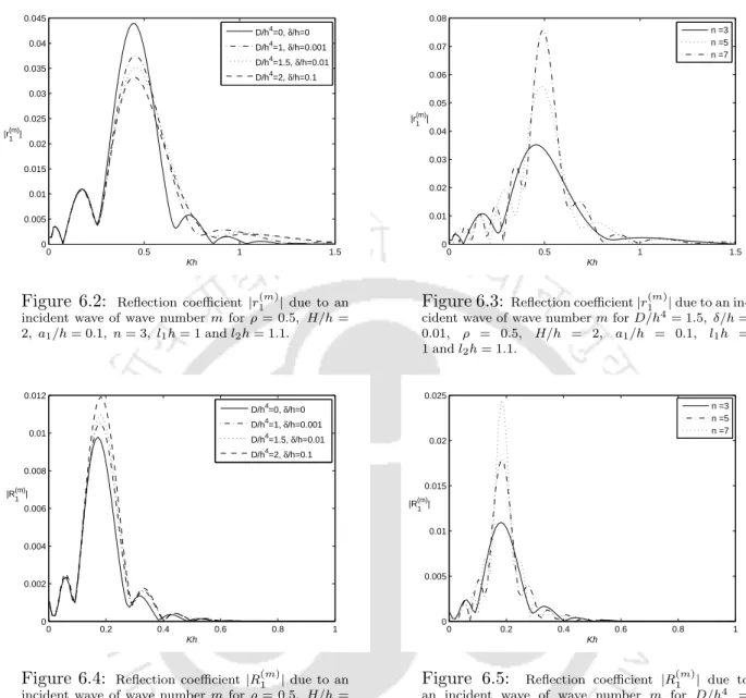
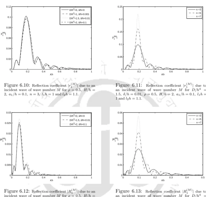
It is clear from these figures (except Figure 6.7) that the peak values of the reflection and transmission coefficients of waves of wavenumbermandM, for the normally incident wave of wavenumbersm, increase as the number of ripples increases. These two figures show that as the values of the ice parameters increase, the maximum values of the reflection and transmission coefficient |r1(M)|and |t(M)1 |, respectively, decrease.
Conclusion
But when the number of ripples becomes very large, the coefficient of reflection and transmission will become unlimited. The reflection and transmission coefficients are approximated to the first order of ε in terms of integrals involving the shape function.
Mathematical formulation of the problem
This occurs due to the presence of the very thin ice cover, which replaces approximately the free surface of the two-layer fluid flow. When they exist, the angle θm of the scattered waves of wavenumberm is given by
Perturbation technique
When the source at (ξ, η), 0< η < H is immersed in the lower fluid, then we consider G1(x, y;ξ, η) and G2(x, y;ξ, η), respectively, as the source potentials in terms of Green's function for the lower and upper layer fluids. Similarly, when the source is immersed in the upper layer of liquid at (ξ, η), −h < η < 0, then we consider G3(x, y;ξ, η) and G4(x, y;ξ, η ), to be the source potentials in terms of Green's function for the lower and upper layer fluids, respectively.
Solution by Green’s function technique
Introduction of Green’s functions
To solve the above coupled boundary value problem described by we need two-dimensional source potentials (in terms of Green's function) for the modified Helmholtz equation due to a source immersed in one of the two layers. Then Green's integral theorem will be used and the first order coefficients r1(m), R(m)1, t(m)1 and T1(m) will be obtained in terms of integrals involving the shape function c(x).
Reflection and transmission coefficients
Solution by Fourier transform technique
Fourier transform technique
M2−ν2, respectively, on the positive real axis of ξ, so the above integral in both cases contains the poles atξ1 and ξ2. Therefore, we make the path for each integral in both cases indented below the poles atξ1 and ξ2.
Reflection and transmission coefficients
Special form of bottom surface
Numerical results
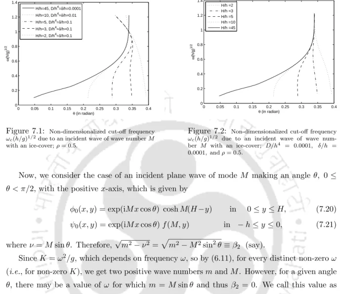
From these figures (except for figure 7.8), it can be seen that the maximum values of reflection and transmission coefficients of waves with wave number m and M for an obliquely incident wave with wave number m increase as the number of waves increases. When θ = 22.5◦, which is greater than the critical angle θc = 22.38◦ for the given values of various parameters Kh, no wave of wave number m propagates in the liquid.
Conclusion
The work described in this chapter is an extension of the work described in Chapter 4. Green's integral theorem is used to obtain the complete solution of the mixed boundary value problem, from which the reflection and transmission coefficients involving a function of the form c(x ) are determined.
Future work
Scattering of water waves from a vertical barrier in each layer of the two-layer liquid covered by the ice sheet. Chakrabarti, To solve the problem of scattering of surface water waves from the edge of an ice sheet, Proc.
Heave added-mass coefficient µ 0 plotted against Ka for a submerged sphere at different ice parameters
Sway added-mass coefficient µ 1 plotted against Ka for a submerged sphere at different depths in lower
Sway added-mass coefficient µ 1 plotted against Ka for a submerged sphere at different ice parameters
Heave damping coefficient ν 0 plotted against Ka for a submerged sphere at different depths in upper
Heave damping coefficient ν 0 plotted against Ka for a submerged sphere at different ice parameters in
Sway damping coefficient ν 1 plotted against Ka for a submerged sphere at different depths in upper
Sway damping coefficient ν 1 plotted against Ka for a submerged sphere at different ice parameters in
Heave added-mass coefficient µ 0 plotted against Ka for a submerged sphere at different depths in upper
Heave added-mass coefficient µ 0 plotted against Ka for a submerged sphere at different ice parameters
Sway added-mass coefficient µ 1 plotted against Ka for a submerged sphere at different depths in lower
Sway added-mass coefficient µ 1 plotted against Ka for a submerged sphere at different ice parameters
Domain definition sketch