Scalable Bayesian Factorization Models for Recommender Systems
A THESIS
submitted by
AVIJIT SAHA
for the award of the degree
of
MASTER OF SCIENCE
(by Research)
DEPARTMENT OF COMPUTER SCIENCE AND ENGINEERING INDIAN INSTITUTE OF TECHNOLOGY, MADRAS.
JUNE 2016
THESIS CERTIFICATE
This is to certify that the thesis titledScalable Bayesian Factorization Models for Rec- ommender Systems, submitted by Avijit Saha, to the Indian Institute of Technology, Madras, for the award of the degree of Master of Science, is a bonafide record of the research work done by him under our supervision. The contents of this thesis, in full or in parts, have not been submitted to any other Institute or University for the award of any degree or diploma.
Dr. B Ravindran Research Guide Associate Professor Dept. of CSE
IIT-Madras, 600 036
Place: Chennai Date: June 08, 2016
ACKNOWLEDGEMENTS
Throughout my stay here, I was fortunate enough to be surrounded by an amazing set of people. I would like to take this opportunity to extend my gratitude to these people. Firstly, I would like to thank my advisor Balaraman Ravindran, who provided me the freedom to explore several areas, and supported me throughout the course. He was more than a teacher and a collaborator from my day one here, a complete mentor. Often I get amazed looking at his diverse knowledge in several domains.
I am charmed to have worked with Professors and colleagues at IIT Madras and else- where, who have been of utmost importance during my education. I would like to thank Ayan Acharya, with whom I have started working towards the end of my course on multi- ple Bayesian nonparametric factorization model problems. He is a fantastic collaborator.
He helped me to get a clear understanding on the recent advances in Bayesian statistics. I would like to thank Ayan Acharya and Joydeep Ghosh for the collaboration which resulted in an ICDM paper. I would also like to thank Rishabh, who worked with me for a long time on Bayesian factorization models. I got a lot of support from him. It was a plea- sure working with Janarthanan and Shubhranshu for the Recsys challenge 2014. I am also thankful to Nandan Sudarsanam for his time on several discussions on bandit problems. I am grateful to Mingyuan Zhou, who gave me the opportunity to collaborate with him on nonparametric dynamic network modeling.
I am largely indebted to my friends without whom I can hardly imagine a single day in the Institute. First of the lot, I would like to thank Saket, with whom I attended several courses. He always stood besides me during my tough days. I am thankful to Animesh and Sai for their support. Also I would like to thank Vishnu, Sudarsan, Aman, Arnab, Ahana, Shamshu, Abhinoy, Vikas, Pratik, Sarath, Deepak, Chandramohan, Priyesh, and Rajkaran for all their help. Thanks to Arpita, Aditya, Viswa, Nandini, Sandhya, and all my 2012 MS friends for making my life at IIT Madras cherishable.
I owe many thanks to my advisor Balaraman Ravindran for helping me to get grants for my research. I am grateful to Ericsson India for funding my research.
Finally, I would like to thank my family for being one of my primary source of inspi- ration, without whom I would not have been able to complete the course. I specially want to thank my mother Shikha Saha, who has supported me always, and has been my biggest strength.
To the memory of my father, Dipak Saha.
ABSTRACT
KEYWORDS: Recommender Systems; Collaborative Filtering; Latent Variable Models; Factorization Models; Matrix Factorization; Factorization Machine; Probabilistic Modeling; Scalable; Bayesian; Variational Bayes; Markov Chain Monte Carlo; Nonparametric.
In recent years, Recommender Systems (RSs) have become ubiquitous. Factorization models are a common approach to solve RSs problems, due to their simplicity, predic- tion quality and scalability. The idea behind such models is that preferences of a user are determined by a small number of unobserved latent factors. One of the most well studied factorization model is matrix factorization using the Frobenius norm as the loss function. In more challenging prediction scenarios where additional “side-information”
is available and/or features capturing higher order may be needed, new challenges due to feature engineering needs arise. The side-information may include user specific features such as age, gender, demographics, and network information and item specific informa- tion such as product descriptions. While interactions are typically desired in such scenar- ios, the number of such features grows very quickly. This dilemma is cleverly addressed by the Factorization Machine (FM), which combines high prediction quality of factor- ization models with the flexibility of feature engineering. Interestingly, the framework of FM subsumes many successful factorization models like matrix factorization, SVD++, TimeSVD++, Pairwise Interaction Tensor Factorization (PITF), and factorized personal- ized Markov chains (FPMC). Also, due to the availability of large data, several sophisti- cated probabilistic factorization models have been developed. However, in spite of having a vast literature on factorization models, several problems exist with different factorization model algorithms.
In this thesis, we take a probabilistic approach to develop several factorization models.
We adopt a fully Bayesian treatment of these models and develop scalable approximate
inference algorithms for them.
Bayesian Probabilistic Matrix Factorization (BPMF), which is a Markov chain Monte Carlo (MCMC) based Gibbs sampling inference algorithm for matrix factorization, pro- vides state-of-the-art performance. BPMF uses multivariate Gaussian prior on latent factor vector which leads to cubic time complexity with respect to the dimension of latent space.
To avoid this cubic time complexity, we develop the Scalable Bayesian Matrix Factoriza- tion (SBMF) which considers independent univariate Gaussian prior over latent factors.
SBMF, which is a MCMC based Gibbs sampling inference algorithm for matrix factoriza- tion, has linear time complexity with respect to the dimension of latent space and linear space complexity with respect to the number of non-zero observations.
We then develop the Variational Bayesian Factorization Machine (VBFM) which is a batch scalable variational Bayesian inference algorithm for FM. VBFM converges faster than the existing state-of-the-art MCMC based inference algorithm for FM while provid- ing similar performance. Additionally for large scale learning, we develop the Online Variational Bayesian Factorization Machine (OVBFM) which utilizes stochastic gradient descent to optimize the lower bound in variational approximation. OVBFM outperforms existing online algorithms for FM as validated by extensive experiments performed on numerous large-scale real world data.
Finally, the existing inference algorithm for FM assumes that the data is generated from a Gaussian distribution which may not be the best assumption for count data such as integer-valued ratings. Also, to get the best performance, one needs to cross-validate over the number of latent factors used for modeling the pairwise interaction in FM, a process that is computationally intensive. To overcome these problems, we develop the Nonpara- metric Poisson Factorization Machine (NPFM), which models count data using the Poisson distribution, provides both modeling and computational advantages for sparse data. The ideal number of latent factors is estimated from the data itself. We also consider a special case of NPFM, the Parametric Poisson Factorization Machine (PPFM), that considers a fixed number of latent factors. Both PPFM and NPFM have linear time and space com- plexity with respect to the number of non-zero observations. Using extensive experiments, we show that our methods outperform two strong baseline methods by large margins.
TABLE OF CONTENTS
ACKNOWLEDGEMENTS i
ABSTRACT iv
ABBREVIATIONS ix
LIST OF TABLES x
LIST OF FIGURES xi
NOTATION xii
1 INTRODUCTION 1
1.1 Contribution of the Thesis . . . 5
1.2 Outline of the Thesis . . . 6
2 BACKGROUND 7 2.1 Recommender Systems . . . 7
2.1.1 Collaborative Filtering . . . 7
2.1.2 Content-based . . . 10
2.1.3 Knowledge-based . . . 10
2.1.4 Hybrid . . . 10
2.2 Latent Variable Models and Factorization Models . . . 11
2.2.1 Matrix Factorization . . . 12
2.2.2 Probabilistic Matrix Factorization . . . 14
2.2.3 Bayesian Probabilistic Matrix Factorization . . . 14
2.2.4 Factorization Machine . . . 16
2.2.5 Learning Factorization Machine . . . 18
2.3 Probabilistic Modeling and Bayesian Inference . . . 20
2.4 Markov Chain Monte Carlo . . . 21
2.4.1 Gibbs Sampling . . . 21
2.5 Variational Bayes . . . 22
2.5.1 Stochastic Variational Inference . . . 24
3 SCALABLE BAYESIAN MATRIX FACTORIZATION 25 3.1 Introduction . . . 25
3.2 Method . . . 28
3.2.1 Model . . . 28
3.2.2 Inference . . . 29
3.2.3 Time and Space Complexity . . . 30
3.3 Experiments . . . 30
3.3.1 Datasets . . . 30
3.3.2 Experimental Setup and Parameter Selection . . . 32
3.3.3 Results . . . 33
3.4 Summary . . . 35
4 SCALABLE VARIATIONAL BAYESIAN FACTORIZATION MACHINE 37 4.1 Introduction . . . 37
4.2 Model . . . 39
4.3 Approximate Inference . . . 40
4.3.1 Batch Variational Inference . . . 40
4.3.2 Stochastic Variational Inference . . . 44
4.4 Experiments . . . 48
4.4.1 Dataset . . . 48
4.4.2 Methods of Comparison . . . 48
4.4.3 Parameter Selection and Experimental Setup . . . 48
4.4.4 Results . . . 49
4.5 Summary . . . 51
5 NONPARAMETRIC POISSON FACTORIZATION MACHINE 53
5.2 Background and Related Work . . . 55
5.2.1 Negative Binomial Distribution . . . 56
5.2.2 Gamma Process . . . 57
5.2.3 Poisson Factor Analysis . . . 57
5.3 Nonparametric Poisson Factorization Machine . . . 58
5.3.1 Model . . . 58
5.3.2 Inference Using Gibbs Sampling . . . 60
5.3.3 Parametric Version . . . 63
5.3.4 Prediction . . . 64
5.3.5 Tme and Space Complexity . . . 65
5.4 Experimental Results . . . 65
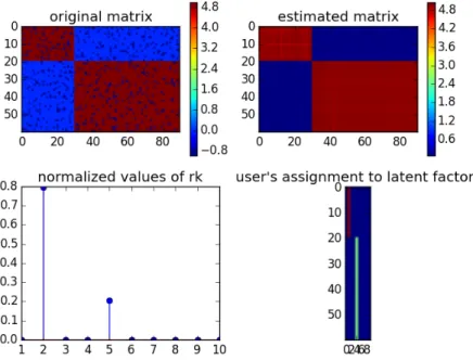
5.4.1 Generating Synthetic Data . . . 65
5.4.2 Simulation . . . 66
5.4.3 Real World Datasets . . . 67
5.4.4 Metric . . . 67
5.4.5 Baseline . . . 69
5.4.6 Experimental Setup and Parameter Selection . . . 70
5.4.7 Results . . . 70
5.5 Summary . . . 72
6 CONCLUSION AND FUTURE WORK 73
ABBREVIATIONS
RSs Recommender Systems
CF Collaborative filtering SVMs Support Vector Machines SGD Stochastic gradient descent MCMC Markov chain Monte Carlo PMF Probabilistic Matrix Factorization
BPMF Bayesian Probabilistic Matrix Factorization FM Factorization Machine
PITF Pairwise Interaction Tensor Factorization FPMC Factorized personalized Markov chains SBMF Scalable Bayesian Matrix Factorization VBFM Variational Bayesian Factorization Machine
OVBFM Online Variational Bayesian Factorization Machine NPFM Nonparametric Poisson Factorization Machine PPFM Parametric Poisson Factorization Machine RMSE Root mean square error
NDCG Normalized Discounted Cumulative Gain IDCG Ideal Discounted Cumulative Gain
LIST OF TABLES
3.1 Time and space complexity comparison between SBMF and BPMF. . . 30
3.2 Description of the datasets for SBMF. . . 33
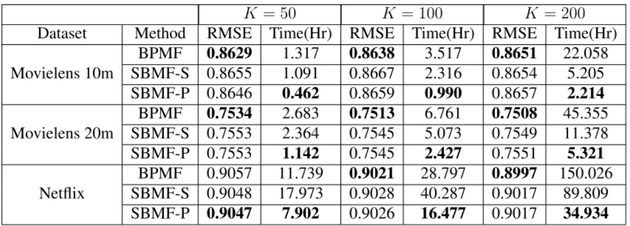
3.3 Results comparison between SBMF and BPMF. . . 34
4.1 Description of the datasets for VBFM and OVBFM. . . 48
5.1 Description of the datasets for NPFM. . . 67
LIST OF FIGURES
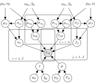
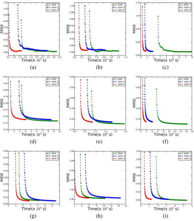
2.1 Feature representation of FM for a song-count dataset with three types of variables: user, song, and genre. . . 17 3.1 Graphical model representation of SBMF. . . 27 3.2 Left, middle, and right columns correspond to the results forK = 50,100,
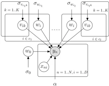
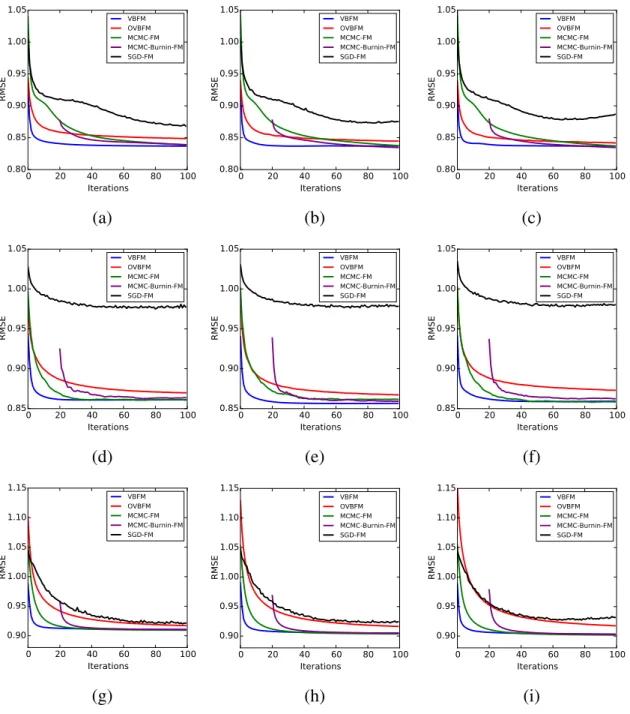
and200respectively. {a,b,c}, {d,e,f}, and {g,h,i} are results on Movielens 10m, Movielens 20m, and Netflix datasets respectively. . . 35 4.1 Graphical model representation of VBFM. . . 40 4.2 Left, middle, and right columns correspond to the results forK = 20, 50,
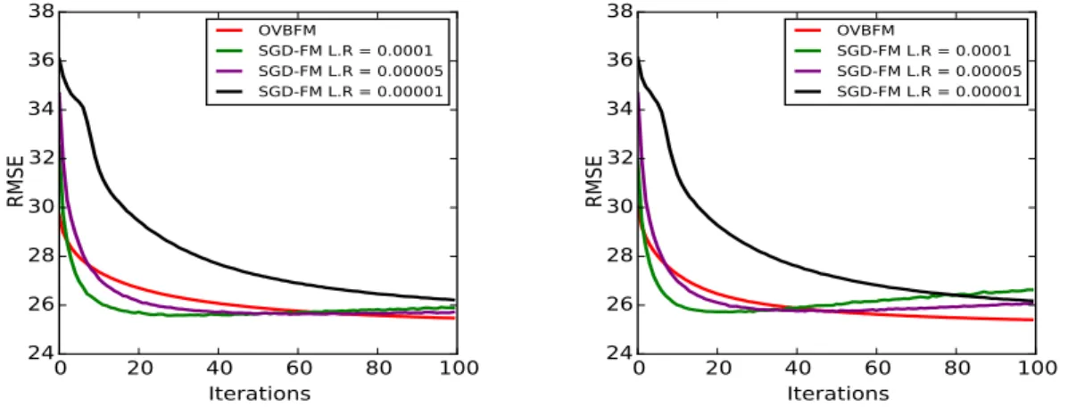
and100respectively. {a,b,c}, {d,e,f}, and {g,h,i} are results on Movielens 1m, Movielens 10m, and Netflix datasets respectively. . . 50 4.3 Left and right columns show results on KDD music dataset for K = 20
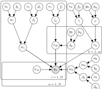
and 50 respectively. . . 51 5.1 Graphical Model representation of NPFM. . . 61 5.2 Results of NPFM on Synthetic dataset. . . 66 5.3 (a), (b), (c), and (d) show Mean Precision, Mean Recall, F-measure, and
Mean NDCG comparison on different datasets for different algorithms re- spectively. . . 69 5.4 (a) and (b) show time per iteration comparison for different algorithms on
Movielens 100k & Movielens 1M and Movielens 10M & Netflix datasets respectively. . . 71
NOTATION
X Matrix
x Column vector, unless explicitly specified as row vector
| Transpose
X.j Summed over index i (i, j) :i < j All(i, j)pairs withi < j
Γ Gamma function
N(·,·) Gaussian distribution Gamma(·,·) Gamma distribution ΓP(·,·) Gamma process
NB(·,·) Negative binomial distribution CRT(·,·) Chinese restaurant table Pois(·,·) Poisson distribution p(·|·) Probability distribution
x∼ Distribution of random variablex
·|− Conditional probability distribution (conditioned on everything except·)
CHAPTER 1
INTRODUCTION
“Information overload occurs when the amount of input to a system exceeds its processing capacity. Decision makers have fairly limited cognitive processing capacity. Consequently, when information overload occurs, it is likely that a reduction in decision quality will occur” - Speier et al. (1999).
Information overload has become a major problem in recent years with the advance- ment of Internet. Social media users and microbloggers receive large volume of informa- tion, often at a higher rate than they can effectively and efficiently consume. Often, users face difficulties in finding relevant items due to the sheer volume of information present in the web, for e.g., finding relevant books from Amazon.com book catalog. Recommender Systems (RSs) and web search help users to systematically and efficiently access informa- tion and help to avoid the information overload problem.
In recent years, RSs have become ubiquitous. RSs provide suggestions of items to users for various decision making processes such as: what song to listen, what book to buy, what movie to watch, etc. Often RSs are built for personalized recommendation and provide user specific suggestions. As few examples: Amazon.com employs a RS to personal- ize the online store for each customer; Netflix provides movie recommendation based on users’ past rating history, current data-query, and users’ profile information; Twitter uses personalized tweet recommendation engine to suggest relevant tweets to users.
Collaborative filtering (CF) [Su and Khoshgoftaar, 2009; Lee et al., 2012; Bell and Koren, 2007] is widely used in RSs and have proven to be very successful. CF takes multiple user’s preferences into account to recommend items to a user. The fundamental assumption of CF is that if two user’s preferences are same on some number of items, then their behavior will be same on the other unseen items. CF [Bell and Koren, 2007] can be viewed as missing value prediction task where given a user-item matrix of scores with
given ones. Memory-based CF algorithms [Su and Khoshgoftaar, 2009] were a common choice in RSs earlier due to their simplicity and scalability. Neighborhood-based (kNN) CF algorithms [Su and Khoshgoftaar, 2009; Bell and Koren, 2007] are prevalent memory- based CF techniques which identify pairs of items that have similar rating behavior or users with similar rating patterns, to find unknown user-item relationship. However memory- based methods are unreliable when the data are sparse [Su and Khoshgoftaar, 2009]. In order to achieve better accuracy and alleviate the short comings of memory-based CF, model-based CF approaches [Hofmann, 2004; Korenet al., 2009; Salakhutdinov and Mnih, 2007] have been investigated.
Model-based CF fits a parametric model to the training data, which is used later to predict the unknown user-item ratings. One particular type of model-based CF algo- rithms is based on latent variable models such as, pLSA [Hofmann, 2004], neural net- works [Salakhutdinov et al., 2007], Latent Dirichlet Allocation [Blei et al., 2003], and matrix factorization [Salakhutdinov and Mnih, 2007] which try to uncover hidden features that explain the ratings. Latent variable models involve supplementing a set of observed variables with additional latent, or hidden, variables. In probabilistic latent variable model framework, the distribution over the observed variables is obtained by marginalizing out the hidden variables from the joint distribution over observed and hidden variables. The hidden structure of the data can be computed and explored through the posterior which is defined as the conditional distribution of the latent variables given the observations. This hidden structure, computed through the posterior distribution, is useful in prediction and exploratory analysis.
Factorization models [Korenet al., 2009; Koren, 2009; Salakhutdinov and Mnih, 2008;
Xionget al., 2010] are a class of latent variable models and have received extensive atten- tion in the RSs community, due to their simplicity, prediction quality, and scalability. These models represent both users and items using a small number of unobserved latent factors.
Hence, each user/item is associated with a latent factor vector. Elements of a item’s la- tent factor measure the extent to which the item possesses those factors and elements of a user’s latent factor measure the extent of interest the user has in items that are high on the corresponding factors. Throughout the thesis, we will adopt a Bayesian approach to
analyze different factorization models.
One of the most well studied factorization model is matrix factorization [Korenet al., 2009; Salakhutdinov and Mnih, 2007, 2008; Gopalan et al., 2015] using the Frobenius norm as the loss function. Formally, matrix factorization recovers a low-rank latent struc- ture of a matrix by approximating it as a product of two low rank matrices. A popular approach to solve matrix factorization is to minimize the regularized squared error loss.
The optimization problem can be solved using stochastic gradient descent (SGD) [Koren et al., 2009]. SGD is an online optimization algorithm which obviates the need to store the entire dataset in memory and hence is often preferred for large scale learning due to mem- ory and speed considerations [Silva and Carin, 2012]. Though SGD is scalable and enjoys local convergence guarantee [Sato, 2001], it often overfits the data and requires manual tuning of the learning rate and the regularization parameters [Salakhutdinov and Mnih, 2007]. On the other hand, Bayesian methods [Salakhutdinov and Mnih, 2008; Beal, 2003;
Tzikaset al., 2008; Hoffmanet al., 2013] for matrix factorization automatically tune learn- ing rate and regularization parameters and are robust to overfitting. Bayesian Probabilistic Matrix Factorization (BPMF) [Salakhutdinov and Mnih, 2008] directly approximate the posterior distribution using Markov chain Monte Carlo (MCMC) based Gibbs sampling inference mechanism and outperform the variational based approximation. BPMF uses multivariate Gaussian distribution as prior on latent factor vector which leads to cubic time complexity with respect to the dimension of latent space. Hence, many times it is difficult to apply BPMF on very large datasets.
In more challenging prediction scenarios where additional “side-information” is avail- able and/or features capturing higher order may be needed, new challenges due to feature engineering needs arise. The side-information may include user specific features such as age, gender, demographics, and network information and item specific information such as product descriptions. While interactions are typically desired in such scenarios, the number of such features grows very quickly. This dilemma is cleverly addressed by the Factorization Machine (FM) [Rendle, 2010], which combines high prediction quality of factorization models with the flexibility of feature engineering. FM represents data as real-valued features as in standard machine learning approaches, such as Support Vec-
tor Machines (SVMs), and uses interactions between each pair of variables as well but constrained to a low-dimensional latent space. By restricting the latent space, the num- ber of parameters needed is kept manageable. Interestingly, the framework of FM sub- sumes many successful factorization models like matrix factorization [Korenet al., 2009], SVD++ [Koren, 2008], TimeSVD++ [Koren, 2009], Pairwise Interaction Tensor Factor- ization (PITF) [Rendle and Schmidt-Thieme, 2010], and factorized personalized Markov chains (FPMC) [Rendle et al., 2011a]. Other advantages of FM include – 1) FM allows parameter estimation with extremely sparse data where SVMs fail; 2) FM has linear com- plexity, can be optimized in the primal and, unlike SVMs, does not rely on support vectors;
and 3) FM is a general predictor that can work with any real valued feature vector, while several state-of-the-art factorization models work only on very restricted input data.
FM is usually learned using stochastic gradient descent (SGD) [Rendle, 2010]. FM that uses SGD for learning is conveniently addressed as SGD-FM in this thesis. As mentioned above, though SGD is scalable and enjoys local convergence guarantees, it often overfits the data and needs manual tuning of learning rate and the regularization parameters. Al- ternative methods to solve FM include Bayesian Factorization Machine [C. Freudenthaler, 2011] which provides state-of-the-art performance using MCMC based Gibbs sampling as the inference mechanism and avoids expensive manual tuning of the learning rate and regu- larization parameters (this framework is addressed as MCMC-FM). However, MCMC-FM is a batch learning method and is less straight forward to scale to datasets as large as the KDD music dataset [Dror et al., 2012]. Also, it is difficult to preset the values of burn-in and collection iterations and gauge the convergence of the MCMC inference framework, a known problem with sampling based techniques.
Also, MCMC-FM assumes that the observations are generated from a Gaussian distri- bution which, obviously, is not a good fit for count data. Additionally, for both SGD-FM and MCMC-FM, one needs to solve an expensive model selection problem to identify the optimal number of latent factors. Alternative models for count data have recently emerged that use discrete distributions, provide better interpretability and scale only with the num- ber of non-zero elements [Gopalanet al., 2014b; Zhou and Carin, 2015; Zhouet al., 2012;
Acharyaet al., 2015].
In this thesis, we take a probabilistic approach to develop different factorization models and build scalable approximate posterior inference algorithms for them. These factoriza- tion models discover hidden structure from the data using the posterior distribution of hidden variables given the observations which is used for prediction purpose.
1.1 Contribution of the Thesis
The contributions of the thesis are as follows:
• Scalable Bayesian Matrix Factorization (SBMF): SBMF considers independent uni- variate Gaussian prior over latent factors as opposed to multivariate Guassian prior in BPMF. We also incorporate bias terms in the model which are missing in baseline BPMF model. Similar to BPMF, SBMF is a MCMC based Gibbs sampling inference algorithm for matrix factorization. SBMF has linear time complexity with respect to the dimension of latent space and linear space complexity with respect to the number of non-zero observations. We show extensive experiments on three large-scale real world datasets to validate that the SBMF takes less time than the baseline method BPMF and incurs small performance loss.
• Variational Bayesian Factorization Machine (VBFM): VBFM is a batch variational Bayesian inference algorithm for FM. VBFM converges faster than MCMC-FM and performs as good as MCMC-FM asymptotically. The convergence is also easy to track when the objective associated with the variational approximation in VBFM stops changing significantly.
• Online Variational Bayesian Factorization Machine (OVBFM): OVBFM uses SGD for maximizing the lower bound obtained from the variational approximation and performs much better than the existing online algorithm of FM that uses SGD. As considering single data instance increases the variance of the algorithm, we consider a mini-batch version of OVBFM.
Extensive experiments on four real world movie review datasets validate the superi- ority of both VBFM and OVBFM.
• Nonparametric Poisson Factorization Machine (NPFM): NPFM models count data using the Poisson distribution which provides both modeling and computational ad- vantages for sparse data. The specific advantages of NPFM include:
– NPFM provides a more interpretable model with a better fit for count dataset.
– NPFM is a nonparametric approach and avoids the costly model selection pro- cedure by automatically finding the number of latent factors suitable for mod- eling the pairwise interaction matrix in FM.
– NPFM takes advantages of the Poisson distribution [Gopalanet al., 2015] and considers only sampling over the non-zero entries. On the other hand, exist-
positive and negative samples in the implicit setting. Such iteration is expen- sive for large datasets and often needs to be solved using a costly positive and negative data sampling approach. NPFM can take advantage of natural sparsity of the data which existing inference technique of FM fails to exploit.
We also consider a special case of NPFM, the Parametric Poisson Factorization Ma- chine (PPFM), that considers a fixed number of latent factors. Both PPFM and NPFM have linear time and space complexity with respect to the number of non- zero observations. Extensive experiments on four different movie review datasets show that our methods outperform two strong baseline methods by large margins.
1.2 Outline of the Thesis
Rest of this thesis is organized as follows:
• Chapter 2 reviews the necessary background work.
• Chapter 3 describes the model and experimental evaluation of SBMF.
• Chapter 4 describes the VBFM and OVBFM and shows their empirical validation.
• Chapter 5 presents the NPFM which can theoretically deal with infinite number of latent factors and evaluation of NPFM on both synthetic and real world dataset. It also analyses a special case of NPFM, the PPFM, that considers a fixed number of latent factors.
• Chapter 6 concludes and explains possible directions for future works.
CHAPTER 2
BACKGROUND
In this chapter, we explain various background works which will be helpful to understand the thesis. We start by discussing Recommender Systems (RSs), followed by latent vari- able models and factorization models. Then we describe a generic probabilistic framework, and using this framework we explain some of the existing Bayesian approximate inference techniques which will be used throughout the thesis.
2.1 Recommender Systems
Recommender Systems (RSs) are software tools and techniques which provide suggestions of appropriate items to users on various decision making processes such as: what song to listen, what book to buy, what movie to watch, etc. But, the appropriate set of items are relative to the individuals. Hence, RSs are often built for personalized recommendation and provide user specific suggestions.
Broadly the RS algorithms can be classified into three categories: 1) collaborative filtering (CF); 2) content-based; and 3) knowledge-based. Combination of these algorithms leads to hybrid algorithms. We provide a brief description of these different types of RS algorithms in this section.
2.1.1 Collaborative Filtering
Collaborative filtering (CF) [Su and Khoshgoftaar, 2009; Leeet al., 2012; Bell and Koren, 2007] is a popular and successful approach to RSs which considers multiple users’ prefer- ences into account to recommend items to a user. The fundamental assumption behind CF is that if two users’ preferences are same on some number of items, then their behavior will
be same on other unseen items. In a typical CF scenario, there is a set of users{1,2, ..., I} and a set of items{1,2, ..., J}, and each user ihas provided preferences/ratings to some number items. This data can be represented as a matrixR ∈ RI×J, whererij is the pref- erence/rating by theith user to thejthitem. The task of the CF algorithm is to recommend unseen items to users. So CF problems can be viewed as missing value estimation task:
estimate the missing values of the matrix R. CF algorithms are generally classified into two categories: memory-based; and model-based.
Memory-based
Memory-based CF algorithms are lazy learners. Neighborhood-based (kNN) CF algo- rithms [Su and Khoshgoftaar, 2009; Bell and Koren, 2007] are most common form of memory-based CF techniques. Earlier, kNN algorithms were mostly user-based approach [Bell and Koren, 2007]. User-based approach estimates the unknown rating of an item for a user based on the ratings of similar users to that item. Formally, to estimate the ratingrij, we consider a set of usersN(i, j), whose rating behavior are similar to useri, and have rated itemj. Here similarity is defined in terms of how two user’s preference behavior match to each other. Then, the estimation of ratingrij is calculated as follows:
ˆrij = ¯ri+ P
i0∈N(i,j)
(ri0j−r¯i0)wii0 P
i0∈N(i,j)
|wii0| , (2.1)
wherer¯i andr¯i0 are the average ratings score of useriand useri0 respectively, andwii0 is the similarity score between useriand useri0. The similarity measure plays an important role, as they are both used to select the members ofN(i, j) and as well as in Eq. (2.1).
Common choices of the similarity measures are Pearson correlation coefficient and cosine similarity. For the user-based algorithm, the Pearson correlation between useriand useri0 is calculated as follows:
wii0 =
P
j∈J0
(rij −r¯i)(ri0j−r¯i0) r P
j∈J0
(rij−r¯i)2r P
j∈J0
(ri0j −r¯i0)2, (2.2)
whereJ0 is the set of items rated by both useriand useri0.
An alternative to user-based approach is item-based approach [Bell and Koren, 2007].
In this method, to predict an unknown ratingrij, we identify a set of itemsN(j, i)that has rating behavior similar to itemj, and userihas rated all the items in the setN(j, i). Then the prediction is done as follows:
rˆij = P
j0∈N(j,i)
rij0wjj0 P
j0∈N(j,i)
|wjj0| , (2.3)
wherewjj0 is the similarity score between itemj and itemj0. The similarity scorewjj0 for item-based approach can be calculated using the Pearson correlation coefficient as follows:
wjj0 =
P
i∈I0
(rij −¯rj)(rij0 −r¯j0) rP
i∈I0
(rij−r¯j)2rP
i∈I0
(rij0 −r¯j0)2
, (2.4)
whereI0 is the set of users who have rated both itemjandj0, andr¯jandr¯j0 are the average rating of itemj andj0 respectively.
Model-based
Though memory-based CF algorithms scale to large data, they are unreliable when the data are sparse [Su and Khoshgoftaar, 2009]. In order to achieve better accuracy and al- leviate the short comings of memory-based CF, model-based CF algorithms [Korenet al., 2009] have been investigated. Model-based CF fits a parametric model to the training data, which later is used to predict the unknown user-item ratings. Model-based methods include cluster-based CF [Connor and Herlocker, 2001; Xue et al., 2005] and Bayesian classi- fiers [Miyahara and Pazzani, 2000]. One widely used and successful type of model-based CF algorithms are based on latent variable models such as, pLSA [Hofmann, 2004], neural networks [Salakhutdinovet al., 2007], Latent Dirichlet Allocation [Bleiet al., 2003], and matrix factorization [Salakhutdinov and Mnih, 2007], which try to uncover hidden features that explain the ratings. Latent variable models involve supplementing a set of observed
framework, the distribution over the observed variables is obtained by marginalizing out the hidden variables from the joint distribution over observed and hidden variables. The hidden structure of the data can be computed and explored through the posterior which is defined as the conditional distribution of the latent variables given the observations.
Factorization models are a widely used model-based CF algorithms which fall under la- tent variable modeling. We will provide detailed discussion on latent variable models and factorization models in Section 2.2.
2.1.2 Content-based
Besides CF, content-based methods [Su and Khoshgoftaar, 2009] are another important class of RS algorithms. Content-based methods make recommendations by analyzing domain knowledge of users and/or items. Typically, content-based methods first extract features of users and/or items and then apply a classification based algorithm to provide recommendations. Unlike CF, content-based methods are limited to the feature informa- tion.
2.1.3 Knowledge-based
Knowledge-based methods [Burke, 2000] use knowledge about users and context, and ap- ply knowledge based techniques to provide recommendation. In knowledge-based meth- ods, users are an integral part of the knowledge discovery process. It uses a knowledge base and develop this base using the user feedback. Knowledge-based methods are par- ticularly helpful when the user wants to give explicit feedback to the system and available user-item interaction data is very less.
2.1.4 Hybrid
There are pros and cons with each type of recommendation algorithms. CF algorithms need a large amount of rating data to provide any useful suggestions. Until there is a large number of users whose habits are known, the system cannot be useful for most users. Also
until a sufficient number of rated items has been collected, the system cannot be useful for a particular user. This problem is known as cold start problem. Similar to CF, content- based methods also suffer from the cold start problem. However, CF and content-based methods are scalable and useful for large datasets. On the other hand, knowledge-based methods avoid cold start problem through user feedback, but suffer from the the prob- lem of costly knowledge base creation process, and hence, less scalable. Hybrid recom- mender [Burke, 2002] systems combine two or more recommendation techniques to gain better performance with fewer of the drawbacks of any individual one. Most commonly, CF is combined with some other techniques. Weighted is a hybridization technique which predicts the score of an item using weighted combination of the prediction from differ- ent recommender algorithms. Another approach is switching between different algorithms using some criterion.
2.2 Latent Variable Models and Factorization Models
A powerful approach to probabilistic modeling involves describing a set of observed vari- ables using a set of latent/hidden variables which is known as latent variable modeling.
Latent variable models are widely used in several domains such as machine learning, statistics, data mining. Latent variable models uncover hidden structure which explains the data. In latent variable models, each observation is associated with a/(a set of) latent variable/variables, therefore, the number of latent variables grows with the size of the data, whereas the number of parameters in a model is usually fixed irrespective of the data size (if latent variables are not part of the parameter set). Latent variable models consider a joint distribution over the hidden and observed variables. Often we seek to find the pos- terior distribution over the hidden variables given the observed variables. Latent Dirichlet Allocation [Bleiet al., 2003] is a well-known example of a latent variable model.
One of the widely used latent variable models in the RSs community are factorization models, due to their simplicity, prediction quality and scalability. The idea behind such models is that preferences of a user are determined by a small number of unobserved latent factors. Matrix factorization [Koren et al., 2009; Salakhutdinov and Mnih, 2007,
2008; Gopalan et al., 2015] is the simplest and most well studied factorization model and has been applied in solving numerous problems related to analysis of dyadic data, such as in RSs [Koren et al., 2009], topic modeling [Arora et al., 2012], and network analysis [Zhou, 2015]. Affinity data between two entities are known as dyadic data. An example of a dyadic data is movie recommendation, where pair of entities involved are user and movie and the affinity response is the rating provided by a user to a movie. Tensor factorization [Xionget al., 2010; Hoet al., 2014; Chi and Kolda, 2012] is an extension of matrix factorization where the data is represented as three dimensional array, signifying interactions of three different variables.
Many specialized factorization models have further been proposed to deal with non- categorical variables. For example, SVD++ [Koren, 2008] uses neighborhood of a user for analysis of movie rating data, TimeSVD++ [Koren, 2009] and Bayesian Probabilistic Tensor Factorization (BPTF) [Xiong et al., 2010] discretize time which is a continuous variable, and factorizing personalized Markov chains (FPMC) [Rendleet al., 2011a] con- siders the purchase history of users to recommend items. Numerous learning techniques have also been proposed for factorization models which include stochastic gradient de- scent (SGD) [Korenet al., 2009], alternating least squares [Zhouet al., 2008], variational Bayes [Lim and Teh, 2007; Kim and Choi, 2014; Silva and Carin, 2012], and Markov chain Monte Carlo (MCMC) based inference [Salakhutdinov and Mnih, 2008].
In this section, we explain some of the important factorization models which will be used throughout the thesis.
2.2.1 Matrix Factorization
Formally, matrix factorization recovers a low-rank latent structure of a matrix by approx- imating it as a product of two low-rank matrices. For delineation, consider a user-movie matrixR∈RI×J whererij cell represents the rating provided to moviejby useri. Matrix factorization decomposes the MatrixRinto two low-rank matricesU = [u1,u2, ...,uI]T
∈RI×K andV = [v1,v2, ...,vJ]T ∈RJ×K, whereui andvj are theK dimensional latent
factor vectors associated with useriand itemj, such that:
R∼U V|. (2.5)
This matrix factorization model is closely related to singular value decomposition, a well-established technique for identifying latent semantic factors in information retrieval.
But applying singular value decomposition with incomplete matrix is undefined and which is often the case in CF. Also addressing only the relatively few known ratings creates over- fitting issue. Earlier methods used imputation to fill the missing entries of the matrix, making the matrix dense. However, these methods are not scalable. Hence recent meth- ods [Korenet al., 2009; Salakhutdinov and Mnih, 2007] model only the observed ratings while avoiding overfitting through regularization. Typically, the latent factors are learned by minimizing a regularized squared error loss function, which is defined as:
X
(i,j)∈Ω
(rij −u|ivj)2+λ ||U||2F +||V||2F
, (2.6)
whereΩis the set of all the observed ratings,λis the regularization parameter and||X||2F
is the Frobenius norm ofX.
Learning
The optimization problem in Eq. (2.6) can be solved using stochastic gradient descent (SGD) [Korenet al., 2009]. In SGD, for each given ratingrij, the update equation of user and item latent factor vectors can be written as follows:
ui ←ui+η 2 rij −uTivj
vj−2λui
, (2.7)
vj ←vj +η 2 rij −uTivj
ui−2λvj
, (2.8)
whereηis the learning rate.
2.2.2 Probabilistic Matrix Factorization
Probabilistic Matrix Factorization (PMF) [Salakhutdinov and Mnih, 2007] provides a prob- abilistic interpretation of matrix factorization. In PMF, factor variables are assumed to be marginally independent whereas rating variables given the factor variables are assumed to be conditionally independent. PMF considers the conditional distribution of the rating variables (the likelihood term) as:
p(R|U,V, τ) = Y
(i,j)∈Ω
N(rij|u|ivj, τ−1), (2.9)
where τ is the precision parameter. Zero-mean spherical Gaussian priors are placed on user and movie latent factor vectors as follows:
U ∼
I
Y
i=1
N(ui|0, λ−1u I), (2.10)
V ∼
J
Y
j=1
N(vj|0, λ−v1I), (2.11)
whereλuandλv are hyperparameters andI is the identity matrix.
The main drawback of this model is that inferring the posterior distribution over the la- tent factors, given the ratings, is intractable. PMF handles this intractability by providing a maximum a posteriori estimation of the model parameters by maximizing the log-posterior over the model parameters, which is equivalent to minimizing Eq. (2.6). So learning PMF model with fixed hyperparameters is equivalent to minimizing Eq. (2.6) which can be done using SGD.
2.2.3 Bayesian Probabilistic Matrix Factorization
Though PMF can be learned using SGD, it suffers from the problem of manual tuning of learning rate and the regularization parameters, and it often overfits the data. One way to solve the problem of manual tuning of regularization parameters is to introduce priors on the hyperparameters and maximize the log-posterior of the model over both parameters
and hyperparameters. Though this method allows automatic model parameter selection, it is not theoretically sound [Salakhutdinov and Mnih, 2008]. So, fully Bayesian Proba- bilistic Matrix Factorization (BPMF) [Salakhutdinov and Mnih, 2008] has been developed which is robust to the overfitting and avoids model selection problem. BPMF considers the likelihood function as in Eq. (2.9) similar to PMF. The prior over user and item latent factor vectors are assumed as:
U ∼
I
Y
i=1
N(ui|µu,Λ−u1), (2.12)
V ∼
J
Y
j=1
N(vj|µv,Λ−v1), (2.13)
where µu,Λu,µv, and Λv are hyperparameters. As Gaussian-Wishart is the conjugate prior of a multivariate Gaussian distribution with unknown mean and precision matrix, Gaussian-Wishart priors are placed on hyperparameters as:
µu,Λu ∼ N(µu|µ0,(β0Λu)−1)W(Λu|W0, ν0), (2.14) µv,Λv ∼ N(µv|µ0,(β0Λv)−1)W(Λv|W0, ν0), (2.15)
whereµ0, β0,W0,andν0 are hyperprior parameters.
Note that a complete conditional is the conditional distribution of a variable given the observations and all other variables in the model, and a conditionally conjugate model is one where each complete conditional has a close distributional form [Hoffman et al., 2013]. As the BPMF model is conditionally conjugate, learning is done using a closed form Gibbs sampling inference mechanism [Salakhutdinov and Mnih, 2008]. Prediction for a ratingrij is done as follows:
rˆij = 1 C
C
X
c=1
(uci)|vcj, (2.16)
whereuci andvcjare thecthdrawn samples for theithuser and thejth item latent factor vec- tors respectively andC is the number of drawn samples from the Gibbs sampling process.
We will describe Gibbs sampling in more detail in Section 2.4.
2.2.4 Factorization Machine
Factorization Machine (FM) combines the advantages of feature based methods like Sup- port Vector Machines (SVMs) with factorization models. Popular feature based methods like SVMs can be learnt using standard tools like LIBSVM [Chang and Lin, 2011] and SVM-Light [Joachims, 2002]. But feature based methods encounter problems when fac- ing high-dimensional but sparse dyadic data where factorization models have been more successful. An FM learns a functionf : RD → T which is a mapping from a real valued feature vectorx ∈ RD to a target domainT. The training data for FM consists ofN tu- ples of the form(xn, yn)Nn=1, wherexnis the feature representation (row vector) andynis the associated response variable for thenth training instance respectively. We will denote y= (y1, y2, ..., yn)andX = (x|1,x|2, ...,x|n)|.
Example
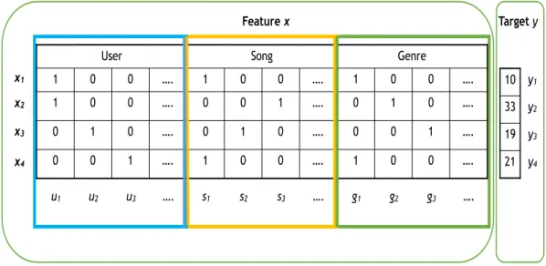
Consider a song-count dataset where the response variable is the number of times a user has listened to a particular song, which has an associated genre. Let us denote user, song, and genre byu, s,andg respectively. If the training data is composed of the set of points {(u1, s1, g1,10),(u1, s3, g2,33),(u2, s2, g3,19),(u3, s1, g1,21)}, then Figure 2.1 shows the corresponding feature representation of FM where the ith column indicates the data cor- responding to the ith variable and the nth row represents the nth training instance. Given the feature representation of Figure 2.1, the model equation for FM for the nth training instance is:
yˆn=w0+
D
X
i=1
xniwi+
D
X
i=1 D
X
j=i+1
xnixnjv|ivj, (2.17) wherew0 is the global bias, wi is the bias associated with theith variable, andvi is the latent factor vector of dimensionKassociated with theith variable.vi|vj models the inter- action between theithandjthfeatures. The objective is to estimate the parametersw0 ∈R, w ∈ RD, and V ∈ RD×K. Instead of using a parameter wi,j ∈ R for each interaction, FM models the pairwise interaction by factorizing it. Since for any positive definite matrix W, there exists a matrixV such that W = V VT provided K is sufficiently large, FM can express any interaction matrixW. This is a remarkably smart way to express pairwise
User Song Genre
1 0 0 …. 1 0 0 …. 1 0 0 ….
1 0 0 …. 0 0 1 …. 0 1 0 ….
0 1 0 …. 0 1 0 …. 0 0 1 ….
0 0 1 …. 1 0 0 …. 1 0 0 ….
x1
x2
x3
x4
10 33 19 21
u1 u2 u3 …. s1 s2 s3 …. g1 g2 g3 ….
Feature x Target y
y1
y2
y3
y4
Figure 2.1: Feature representation of FM for a song-count dataset with three types of vari- ables: user, song, and genre. An example of four data instances are shown.
Row 1 shows a data instance where user u1 listens to songs1 of genre g1 10 times.
interaction in big sparse datasets. In fact, many of the existing CF algorithms aim to do the same, but with the specific goal of user-item recommendation and thus fail to recognize the underlying mathematical basis that FM successfully discovers.
Interestingly, the framework of FM subsumes many successful factorization models like matrix factorization [Koren et al., 2009], SVD++ [Koren, 2008], TimeSVD++ [Ko- ren, 2009], Pairwise Interaction Tensor Factorization (PITF) [Rendle and Schmidt-Thieme, 2010], and factorized personalized Markov chains (FPMC) [Rendleet al., 2011a], and has also been used for context aware recommendation [Rendle et al., 2011b]. Other advan- tages of FM include – 1) FM allows parameter estimation with extremely sparse data where SVMs fail; 2) FM has linear complexity, can be optimized in the primal and, unlike SVMs, does not rely on support vectors; and 3) FM is a general predictor that can work with any real valued feature vector, while several state-of-the-art factorization models work only on very restricted input data.
2.2.5 Learning Factorization Machine
Three learning methods have been proposed for Factorization Machine (FM): 1) stochastic gradient descent (SGD) [Rendle, 2010], 2) alternating least squares (ALS) [Rendleet al., 2011b], and 3) Markov chain Monte Carlo (MCMC) [C. Freudenthaler, 2011] inference.
Here, we will briefly describe SGD and MCMC learning for FM.
Optimization Task
Optimization function for FM with L2 regularization can be written as follows:
X
(xn,yn)∈Ω
l(ˆyn, y) +X
θ∈θ
λθθ2, (2.18)
whereΩis the training set, θ = {w0,w,V}, λθ is the regularization parameter, andl is the loss function. For binary observations, the loss function is assumed to be a sigmoid and for other cases, it is assumed to be a square loss.
Probabilistic Interpretation
Both loss and regularization can be motivated from a probabilistic point of view. For least squares loss, the target y follows a Gaussian distribution.
yn∼ N(ˆyn, α−1), (2.19)
whereαis the precision parameter. For binary classification, y follows a Bernoulli distri- bution.
yn ∼Bernoulli(b(ˆyn)), (2.20)
where b is a link function. L2 regularization corresponds to Gaussian prior on the model parameters.
θ∼ N(µθ, σ−1θ ), (2.21)
whereµθandσθare hyperparameters.
Stochastic Gradient Descent
One of the more popular learning algorithms for FM is based on stochastic gradient descent (SGD). FM that uses SGD for learning is conveniently addressed as SGD-FM. Algorithm 1 describes the SGD-FM algorithm. SGD-FM requires costly search over the parameter space to find the best values for the learning rate and the regularization parameters. To mitigate such expensive tuning of parameters, learning algorithm based on ALS have also been proposed to automatically select the learning rate.
Algorithm 1Stochastic Gradient Descent for Factorization Machine (SGD-FM) Require: Training dataΩ, regularization parametersλ, learning rateη, initializationσ.
Ensure: w0 ←0,w←(0, ...,0), vik ∼ N(0, σ−1).
1: repeat
2: for(xn, yn)∈Ωdo
3: w0 ←w0−η
∂
∂w0l(ˆyn, yn) + 2λ0w0
4: fori= 1toD∧xni 6= 0do
5: wi ←wi−η
∂
∂wil(ˆyn, yn) + 2λiwi
6: fork = 1toK do
7: vik ←vik−η
∂
∂vikl(ˆyn, yn) + 2λikvik
8: end for
9: end for
10: end for
11: untilconvergence
Markov Chain Monte Carlo
As an alternative, Markov chain Monte Carlo (MCMC) based Gibbs sampling inference has been proposed for FM. FM that uses MCMC for learning is conveniently addressed as MCMC-FM. MCMC-FM is a generative approach. In MCMC-FM, tuning of parameters is less of a concern, yet it produces state-of-the-art performance for several applications.
MCMC-FM considers the conditional distribution of the rating variables (the likelihood term) as:
p(y|X,θ, α) = Y
(xn,yn)∈Ω
N(yn|yˆn, α−1) (2.22)
MCMC-FM assumes priors on the model parameters as follows:
w0 ∼ N(w0|µ0, σ0−1), (2.23) wi ∼ N(wi|µi, σi−1), (2.24) vik ∼ N(vik|µik, σik−1), (2.25)
α ∼ Gamma(α|α0, β0). (2.26)
On each pair of hyperparameters (µi, σi) and (µik, σik) ∀i, k a Gaussian distribution is placed onµand a gamma distribution is placed onσas follows:
µi ∼ N(µi|µ0,(ν0σi)−1), (2.27) σi ∼ Gamma(σi|α00, β00), (2.28) µik ∼ N(µik|µ0,(ν0σik)−1), (2.29) σik ∼ Gamma(σik|α00, β00), (2.30)
whereµ0, ν0, α00,andβ00 are hyperprior parameters.
MCMC-FM is a closed form Gibbs sampling inference algorithm for the above model.
Please refer to [C. Freudenthaler, 2011] for more detailed analysis on MCMC-FM infer- ence equations.
2.3 Probabilistic Modeling and Bayesian Inference
Here we will explain a general probabilistic framework, by which we will describe some of the existing approximate inference techniques. AssumeX = (x1,x2, ...,xN)∈RD×N are the observations andθ is the set of unknown parameters for the model that generates X. For example, assuming X is generated by a Gaussian distribution, θ would be the mean and the variance of that Gaussian distribution. One of the most popular approaches for parameter estimation is maximum likelihood. In maximum likelihood, the parameters are estimated as:
θˆ=argmaxθp(X|θ) (2.31)
The generative model may also include latent or hidden variables. We will denote hidden variables by Z. These random variables act as links, that connect the observations to the unknown parameters, and help to explain the data. Given this set up, we aim to find the posterior distribution of latent variables which is written as follows:
p(Z|X,θ) = p(X|Z,θ)p(Z|θ)
p(X|θ) (2.32)
= p(X|Z,θ)p(Z|θ) R
Zp(X|Z,θ)p(Z|θ)dZ (2.33) But often the denominator in Eq. (2.33) is intractable and hence we need to resort to some approximate inference techniques to calculate the posterior distribution approxi- mately. We explain two popular approximate inference techniques in details below which are used in this thesis.
2.4 Markov Chain Monte Carlo
Markov chain Monte Carlo (MCMC) methods [Metropolis and Ulam, 1949; Hastings, 1970] are established tools for solving intractable integration problems central to Bayesian statistics. MCMC method was first proposed by Metropolis and Ulam in 1949 [Metropolis and Ulam, 1949] and then generalized to Metropolis-Hastings method [Hastings, 1970].
MCMC method constructs a Markov chain with state spaceZandp(Z|X,θ)as stationary distribution to sample fromp(Z|X,θ). The simulated values can be considered as coming from the target distribution if the chain is run for long time. A Markov chain is generated by sampling for a new state of the chain depending on the present state of the chain, ignoring all the past states.
2.4.1 Gibbs Sampling
Gibbs sampling [Geman and Geman, 1984; Gelfand and Smith, 1990] is the most widely applied MCMC method. Gibbs sampling is a powerful tool when we cannot sample di- rectly from the joint-posterior distribution, but when sampling from the conditional distri-
butions of each variable, or set of variables, is possible. Gibbs sampling aims to generate samples from the posterior distribution ofZthat is partitioned intoMdisjoint components Z = (Z1,Z2, ...,ZM). Although it may be hard to sample from the joint-posterior, it is assumed that it is easy to sample from the full conditional distribution of Zi. Initially all the parameters are initialized by random values and then the sampling process goes as follows:
Z1(t+1)|− ∼p
Z1|X,θ,Z2(t),Z3(t), ...,ZM(t) Z2(t+1)|− ∼p
Z2|X,θ,Z1(t+1),Z3(t), ...,ZM(t) Z3(t+1)|− ∼p
Z3|X,θ,Z1(t+1),Z2(t+1),Z4(t), ...,ZM(t) ...
whereZitis the sample drawn for theith component in thetth iteration. For more detailed discussion on MCMC methods look into [Metropolis and Ulam, 1949].
2.5 Variational Bayes
Variational methods have their origins on the calculus of variations. Unlike standard calcu- lus, variational calculus considers functional which is defined as a mapping which takes as input a function and output the value of the functional. The functional derivative is defined as the change of the functional for the small change in the input function. Variational in- ference, an alternative to MCMC sampling, transforms a complex inference problem into a high-dimensional optimization problem [Beal, 2003; Tzikaset al., 2008; Hoffmanet al., 2013]. It explores all possible input functions to find the one that maximizes, or minimizes, the functional.
Variational inference optimizes the marginal likelihood function. For our framework, the marginal likelihood function can be written as follows:
lnp(X|θ) =L(q,θ) +KL(q||p), (2.34)
where,
L(q,θ) = Z
Z
q(Z) ln
p(Z,X|θ) q(Z)
dZ, (2.35)
KL(q||p) =− Z
Z
q(Z) ln
p(Z|X,θ) q(Z)
dZ, (2.36)
whereq(Z)is any probability distribution. KL(q||p)is the Kullback-Leibler divergence between q(Z) and p(Z|X,θ), and is always non-negative. Thus lnp(X|θ) is lower- bounded by the term L(q,θ), also known as evidence lower bound (ELBO) [Beal, 2003;
Tzikas et al., 2008]. We can maximize the lower bound L(q,θ) by optimization with respect to the distribution q(Z), which is equivalent to minimizing the KL divergence.
Maximum of the lower bound occurs when KL divergence vanishes, which occurs when q(Z) equal top(Z|X, θ). However, in practice working with the true posterior distribu- tion is intractable. Therefore, a restrictive form ofq(Z)is considered, and then a member of this family is found which minimizes the KL divergence. Typically, a factorized distri- bution is considered of the hidden variablesZwhich factorizes intoM disjoint partitions.
Also it is assumed thatq(Z)factorizes with respect to these partitions as follows:
q(Z) =
M
Y
i=1
qi(Zi) (2.37)
Among all distributions q(Z)with the form Eq. (2.37), we want to find the distribution for which the lower bound is largest. A free form optimization is performed of L(q,θ) with respect to all of the distributionsqi(Zi), which is done by each factors in turn. Let us considerqj(Zj)asqj and using Eq. (2.37) lower bound can be written as:
L(q,θ) = KL(˜p||qj)−X
i6=j
Z
qilnqidZi, (2.38)
where,
ln ˜p(X,Zj|θ) =Ei6=j[lnp(X,Z|θ)] +const (2.39) Now keeping{qi6=j} fixed and maximization of lower bound with respect to all possible distributions of qj(Zj) is equivalent to minimizing KL divergence in Eq. (2.38). So we
get:
lnqj∗(Zj) = ln ˜p(X,Zj|θ) = Ei6=j[lnp(X,Z|θ)] +const (2.40) The constant term can be calculated using normalization.
qj∗(Zj) = exp (Ei6=j[lnp(X,Z|θ)])
R exp (Ei6=j[lnp(X,Z|θ)])dZj (2.41)
In summary, the variational EM algorithm can be written as:
E-Step: EvaluateqNEW(Z)to maximizeL(q,θ)solving the system of Eq. (2.41).
M-Step: FindθNEW =argmaxθL(q,θ).
Note, that here we do not consider the form of qj(Zj), they are found automatically.
Also, the lower bound provides another way to approach the variational inference. If the functional form of the factors in the variational posterior distribution are known, then by taking general parametric form of these distributions, we can write the lower bound. Then we can maximize the lower bound with respect to these parameters by setting the derivative of lower bound with respect to these parameters to zero, which gives the re-estimation equations. For more detailed and introductory discussion on variational Bayes look into [Bishop, 2006; Tzikaset al., 2008; Beal, 2003].
2.5.1 Stochastic Variational Inference
Recently stochastic variational inference has been applied in many places such as, stochas- tic variational inference (SVI) in matrix factorization [Hernández-Lobato et al., 2014], topic modeling [Hoffman et al., 2013] and network modeling [Gopalan et al., 2012].
Specifically, SVI samples a complete data instance, such as a document, and updates all the model parameters. Often, to reduce the variance instead of sampling a single data point to update the parameters, a batch of points are sampled and then the variational parameters associated to this batch of data points are updated. This version of variational inference is called as mini-batch variational inference [Hoffmanet al., 2013].
CHAPTER 3
SCALABLE BAYESIAN MATRIX FACTORIZATION
Bayesian Probabilistic Matrix Factorization (BPMF), which is a Markov chain Monte Carlo (MCMC) based Gibbs sampling inference algorithm for matrix factorization, pro- vides state-of-the-art performance. BPMF uses multivariate Gaussian prior on latent factor vector which leads to cubic time complexity with respect to the dimension of latent space.
To avoid this cubic time complexity, in this chapter, we develop the Scalable Bayesian Matrix Factorization (SBMF) which considers independent univariate Gaussian prior over latent factors. We also incorporate bias terms in the model which are missing in baseline BPMF model. Similar to BPMF, SBMF is a MCMC based Gibbs sampling inference al- gorithm for matrix factorization. SBMF has linear