I am happy to thank Indian Institute of Technology Guwahati and Council of Scientific and Industrial Research (CSIR) for providing scholarship during my Ph.D. The idea of an adaptive network is then extended for the first time in the literature in Chapters 4 and 5 to solve singularly perturbed differential-difference equations with delay and moving terms.
Singular Perturbation Problem
A direct numerical solution of the SPP is difficult due to the presence of a thin boundary layer. As a result, not all boundary or initial conditions can be satisfied by the perturbation expansion.
Objective and Motivation
Many researchers used finite difference methods to approximate the unweighted and ε-weighted (in the literature, also known as the normalized flux) derivatives of the solution. But their analysis based on the direct expansion of the antiwind solution turns out to be complicated.
Preliminaries
The analysis uses the standard supremum normk · kork · kD, which is defined by. Further discussion on the choice of standard can be found in the book by Miller et al.
Model Problems
Singularly perturbed convection-diffusion Dirichlet boundary-value problems 10
Singularly perturbed delay differential equations
Singularly perturbed differential-difference equations
Here we follow the same technique as in and expand the delay and displacement terms through a Taylor series expansion assuming a sufficient smoothness condition on the solution (1.4.4) so that BVP (1.4.4) reduces to a standard singular perturbation problem.
Outline of the Thesis
The defect correction method combines the stability of the upwind scheme and the higher-order convergence of the central difference scheme. The convergence of the global solution via interpolation and the error in the global normalized flux are also discussed in the same section.
Continuous Problem
The estimates for the local truncation error, the bounds for the weighted derivative errors and the convergence analysis of the numerical solution obtained by the headwind scheme on the adaptive grid are proven in Section 2.5.
Generation of Nonuniform Grids
The Shishkin mesh
Now in each subdomain a uniform mesh with N/2 mesh intervals is placed so that the piecewise uniform mesh is of the form. One can note that the piecewise uniform mesh reduces to a uniform mesh if σ = 1/2, which occurs when N ≥exp(α/2ε).
The adaptive grid
A desirable property of the monitor function is that there exist some positive constants C1≤C2 such that. To simplify the treatment, we construct the monitor function (2.3.3) from the exact solution of (2.1.1).
Practical implementation
In other words, find{xi, uNi } with{uNi }calculated from the{xi} using the discrete scheme (2.4.1), so that. You can refer to more details about the adaptive algorithms and their stopping criterion. Existence of a solution to the equilibrium distribution problem) For any ε∈(0,1] and any positive integer N, there exists a mesh that provides a solution to the equilibrium distribution problem that evenly distributes the discrete arc length monitor function of (2.3.7). for the model problem (2.1.1).
Discrete Problem
Error Analysis
- Local truncation error
- Convergence of the numerical solution
- Error in the normalized flux
- Convergence of the global solution
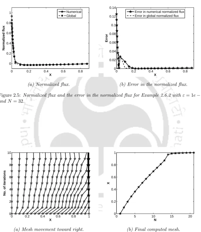
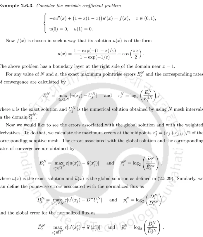
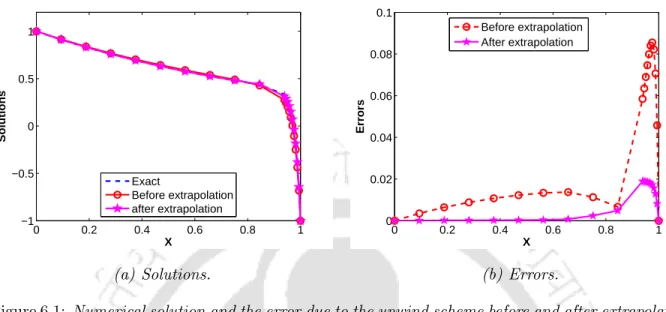
The limit for the weighted error ε between the calculated derivative and the actual one of the solution of (2.1.1) is given in the following theorem. Figure 2.6(a) shows the movement of the mesh to the right and the final mesh is shown in Figure 2.6(b).
Conclusion
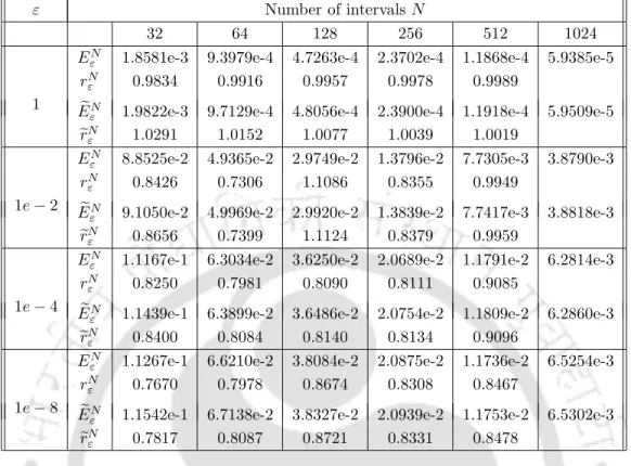
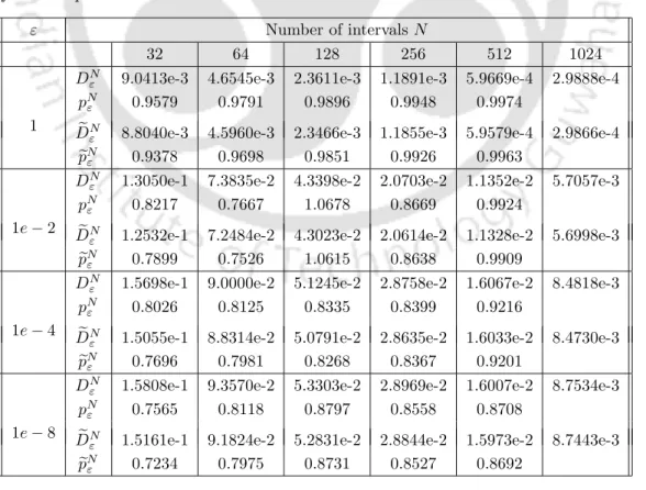
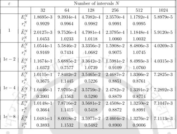
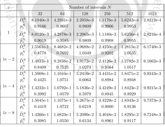
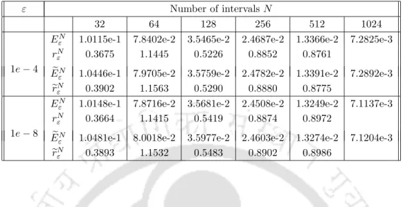
In Table 2.1 and Table 2.2, the maximum point error and the corresponding order of convergence for the solution and its derivative, respectively, are presented for Example 2.6.1. Similar results are shown in Table 2.3 and Table 2.4 for Example 2.6.2, which clearly show that the proposed method is e-uniformly convergent of order 1.
Continuous Problem
The convergence analysis of the numerical solution obtained by the headwind scheme is discussed in Section 3.4. In the next lemma we obtain bounds for the components of the solution and their derivatives.
Numerical Scheme and Nonuniform Grids
Discrete problem
Note that ifk=N, then D−VN ≤0 and also VN < 0, which violates the right-hand side boundary condition and thus k 6=N. To avoid this contradiction, we can take Vk =Vk−1 = Vk+1 <0, which is again a contradiction to the right-hand side boundary condition.
Grid equidistribution
In the tri-diagonal system (3.3.3), off-diagonal entries have the following properties: Discrete Comparison Principle) Let LN be the finite difference upwind operator as defined in (3.3.1) and letΩN be an arbitrary mesh of N+ 1 mesh points. The system of equations (3.3.1) and (3.3.6) are solved simultaneously to obtain the solution UjN and nettxj.
Error Analysis
Local truncation error
Now consider the case when the network is non-uniform, then the solution has the form Φj = µNj −j+ (λ2α/λ1ε)−1. The above error estimates for the regular and singular component of the numerical solution now lead to the following error estimate.
Numerical Results
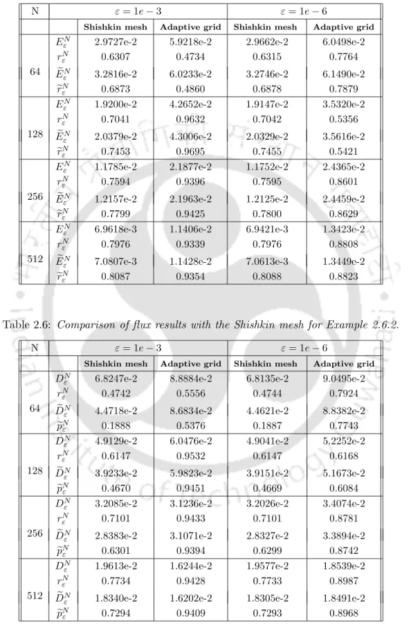
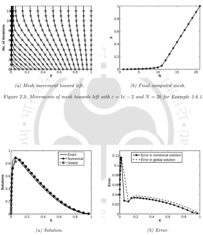
Figures 3.1(a) and 3.1(b) present the numerical solution together with the exact solution and the corresponding error obtained on the adaptive mesh for Case 3.5.1. Computational results using an adaptive grid are compared with numerical results using a Shishkin grid and are shown in Table 3.2 with ε= 1e−3 and ε= 1e−6 for case 3.5.1.
Conclusion
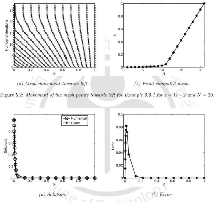
The numerical solution of BVP (4.1.10) with a large number of mesh points is treated as the exact solution of the original BVP (4.1.1). The numerical solution obtained by the proposed method is compared with the numerical solution of BVP (4.1.10).
Continuous Problem
Properties of the solution and its derivatives
A bound on the local truncation error is obtained in Section 4.4 and the error analysis is performed leading to the main theoretical result, namely ε-uniform convergence to the maximum norm. Finally, some numerical examples are given in Section 4.5 to illustrate the applicability of the present method with the maximum point error and the convergence rate are presented in terms of tables and figures.
Discrete Problem
The difference scheme
By following the technique of [28] for the one-parameter problem, we can obtain the required result.
Grid equidistribution
Error Analysis
Local truncation error
Using the bottom of the derivative of the continuous solution (4.2.2) in the first term, the above expression can be written as.
Bound on maximum point-wise error
Now we can repeat the same argument by replacing ej with −ej, and thus we have
Layer on the right side
Let us apply the discrete comparison principle as given in Lemma 4.4.2 to the barrier function Wj. Here it is essential to observe that one can construct the nonuniform mesh as given in (4.3.5) through the same monitor function defined in (4.3.4) in the case of the right boundary layer without any extra care.
Numerical Results
Table 4.2 and Table 4.4 present the maximum point error and the corresponding order of convergence for cases 4.5.1 and 4.5.3, respectively. The maximum point error and the corresponding order of convergence for Cases 4.5.2 and 4.5.4 are given in Tables 4.3 and 4.5, respectively.
Conclusion
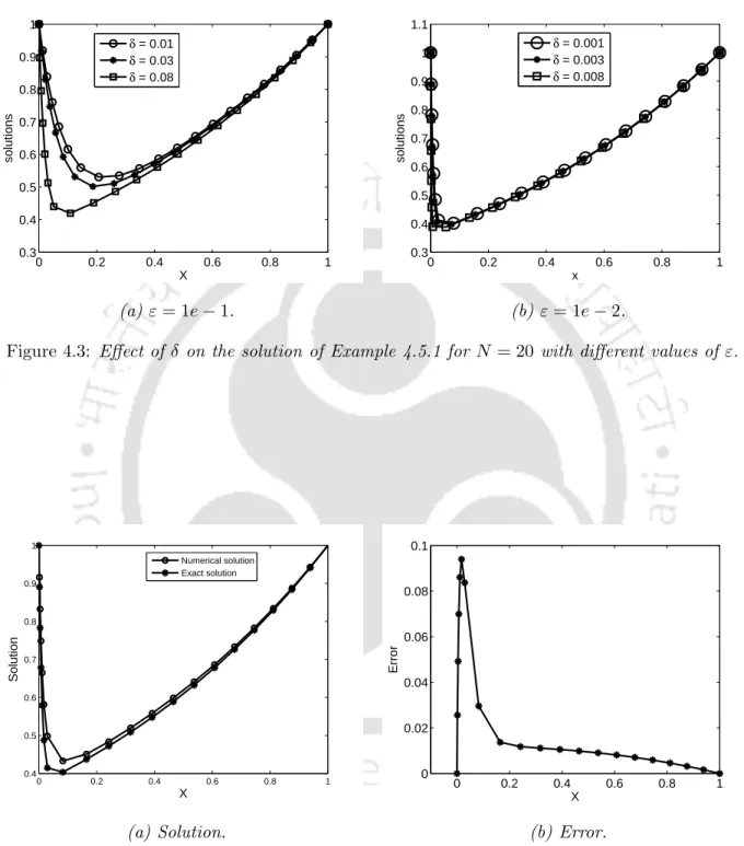
If the delay and the shift are small enough, one can expect u(x) to give a good approximation to uε(x). To calculate the maximum pointwise error EbεN and the rate of convergence brεN, the idea of interpolation is used.
Continuous Problem
The bounds for the local truncation error and for the maximum pointwise error are obtained in section 5.4. Finally, in Section 5.5, several numerical examples are given to illustrate the applicability of the proposed method.
Discrete Problem
Adaptive grid
The adaptive grid can be constructed as the solution of the following non-linear system of equations:
Error Analysis
Local truncation error
The main result, namely, the ε-uniform convergence of the upwind scheme is given in the following theorem. This assumption implies that the boundary layer occurs in the vicinity of x= 1, i.e., on the right side of the interval.
Numerical Results
Here it is significant to observe that the non-uniform mesh as given in (5.3.5) can be constructed by the same monitor function as defined in (5.3.4) in the case of the right boundary layer. Similarly, the equation for Example 5.5.2 is also shown in Table 5.6 in the case of the right boundary layer.
Conclusion
Then the Richardson extrapolation technique is applied to the calculated solution which establishes the transition parameter of the Shishkin mesh. Then, by a simple post-processing technique to improve the rate of convergence of the order O(N−2ln2N).
Continuous Problem
Properties of the solution and its derivatives
Finally, some numerical examples are provided in Section 6.5 to illustrate the applicability of the present method and the maximum pointwise error and the corresponding convergence rate are shown in terms of tables and figures. By differentiating (6.1.3) twice and following the same argument given in Chapter 4, one can obtain the result for k= 4,5.
Solution decomposition
By applying the maximum principle as given in Lemma 6.2.1, we can thus conclude that ψ±(x)≥ 0,∀x ∈Ω and thus the required result. To obtain the necessary bound on w(x) and its derivative, we consider the barrier function ψ±(x) =Cexp.
Discrete Problem
The Shishkin mesh
The upwind scheme
Convergence of the upwind scheme
The discrete solution UN is decomposed as UN =VN +WN, where VN is the solution of the BVP. Now by combining the error bounds of the regular component given in (6.3.12) and the simple component given in (6.3.13), we get the required result.
Richardson Extrapolation Technique
In the next lemma we get the second-order error bound for the extrapolation of the singular component. The main result of this chapter is stated in the following theorem, which provides the ε-uniform second-order convergent result of the Richardson extrapolation technique applied to the BVP (6.1.3).
Numerical Results
Table 6.1 presents the maximum point errors before and after extrapolation for a range of ε and N values and the corresponding order of convergence. The maximum point error and the corresponding order of convergence for Example 6.5.2 are given in Table 6.2.
Conclusion
Clearly, these figures show that the calculated errors decrease at approximately the same rates as proven theoretically, and the rate of convergence of the upwind scheme doubles after extrapolation. From these calculation results, one can observe the ε-uniform convergence of the scheme before and after extrapolation.
Continuous Problem
Properties of the solution
Under these assumptions, the BVP (7.1.3) has a unique solution which exhibits an exponential layer on the right-hand side of the domain at x = 1. In Section 7.2, the maximum principle, the stability result, and some a priori estimates on the solution and derivatives of of GDP (7.1.3) are established.
Solution decomposition
Discrete Problem
- The Shishkin mesh
- The difference scheme
- Convergence of the upwind scheme
- Decomposition of the discrete solution
The local truncation error of the difference scheme (7.3.1) at the node xi is given by. It also follows that LNupξ(xi)<0 and LNcdξ(xi)<0, so using the discrete equation principle (Lemma 7.3.1).
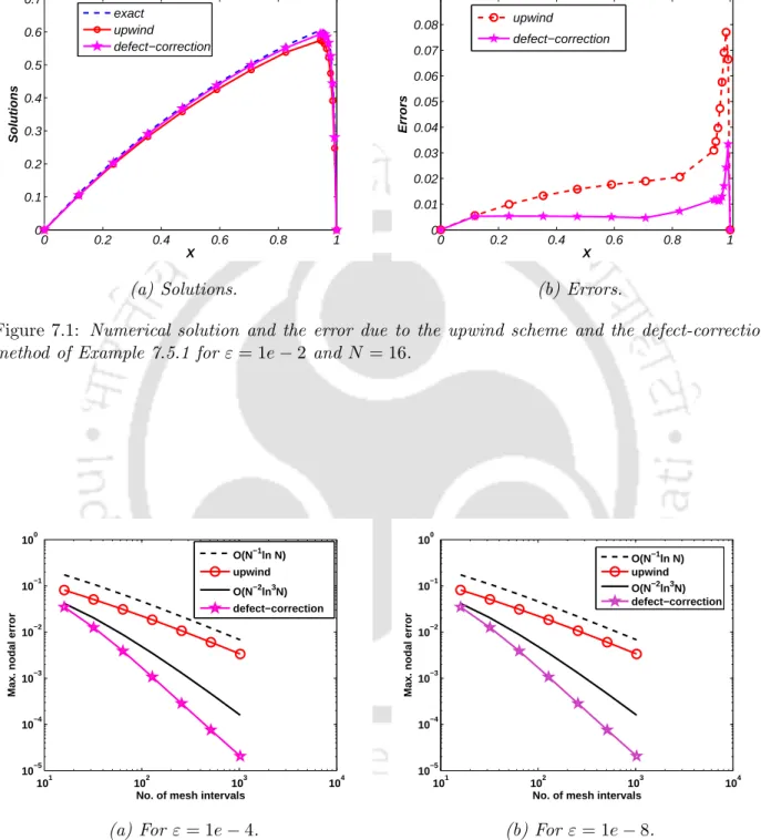
The Defect-Correction Method
Now we will find the truncation error in the regular component of the debug method. We are now in the troubleshooting phase of the regular part of the debugging method. 7.4.23).
Numerical Results
In Table 7.1, the maximum point errors and the corresponding order of convergence of the upwind scheme and error correction method are shown for a range of values of ε and N. The maximum point errors and the corresponding order of convergence for Example 7.5.2 are given in table 7.2.
Conclusion
Clearly, these figures show that the calculated errors decrease at roughly the same rates as theoretically validated, and the convergence rate of the upwind scheme almost doubles using the error correction method. It is shown theoretically and numerically that by using the error correction method, the convergence rate of the upwind scheme increases from almost first order to almost second order.
Future Scopes
An ε-uniform equipped operator method for solving boundary value problems for singularly perturbed differential equations with delay: layer behavior. A finite difference based numerical method for boundary value problems for singularly perturbed differential equations with delay.