Current emissions and speed measurements were carried out on the test track with the integration of an autogas analyzer and V–Box1. The study measured peak and off-peak tailpipe emissions of passenger cars and auto-rickshaws and analyzed them against different mileages with current speed and acceleration for interrupted and congested traffic conditions.
GENERAL 1
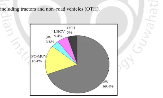
The proportion of passenger cars and auto-rickshaws (three-wheelers) on city roads is high in India. Auto-rickshaws are the popular form of private transport due to the low initial cost and low operating cost (Iyer, 2003).
URBAN TRAFFIC EMISSION AND AIR QUALITY 4
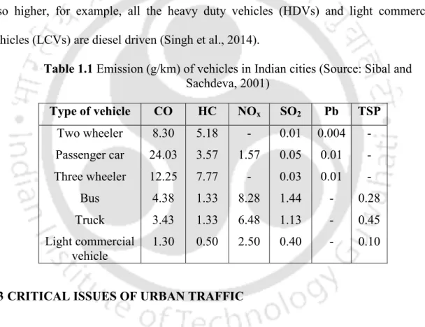
Emissions of CO and HC are high for personalized modes (e.g. cars and 2W) and para-transit modes (e.g. 3W) compared to buses and trucks.
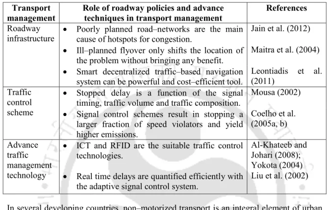
CRITICAL ISSUES OF URBAN TRAFFIC 5
Traffic interruption and congestion 6
Traffic congestion that causes stop delay and approach delay4 increases the total travel time and consequently increases the fuel consumption (Pandian et al., 2009). The management of traffic demand and supply is responsible for traffic congestion (Arnott et al., 1991).
Traffic emission due to interruption and congestion 8
2011a, b) also reported that autorickshaws with two-stroke engines had a share of about 20%. higher fuel consumption and CO2 emissions, and a much greater chance of being categorized as having high particulate matter emissions than those with four-stroke engines. Within the group of four-stroke vehicles, age is a very important predictor, with older models more likely to cause high PM emissions.
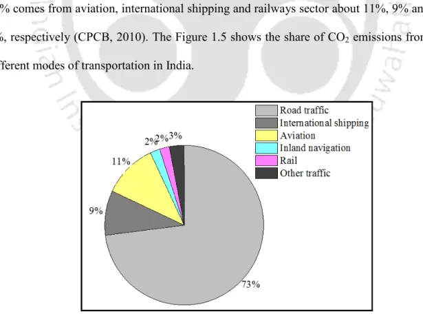
Greenhouse gases emission 10
RESEARCH OBJECTIVE 11
Work plan 11
Correlation study of travel time fraction and speed versus co-emission.
NOVELTY OF THE RESEARCH 12
ORGANIZATION OF THE THESIS 12
This discrepancy has further increased with the increase in mileage of passenger cars and auto-rickshaws. It was assumed that the state of the traffic flow is similar in both directions of the road section.
LITERATURE REVIEW 15-36
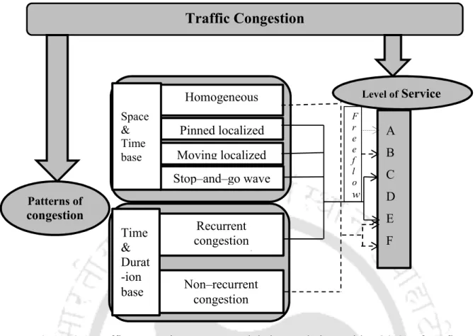
PATTERN OF TRAFFIC CONGESTION 15
Traffic congestion patterns are also defined based on duration and timing and are named as recurring and non-recurring congestion (Dowling et al., 2004; Varaiya, 2007). Level of service (LOS) is another scale used to determine the level of traffic flow (Mannering et al., 2007).
CHARACTERISTICS OF TRAFFIC CONGESTION 18
- Road characteristics 19
- Traffic composition and roadway capacity 19
- Traffic planning and management 21
- Driving behaviour 23
The traffic composition is uncertain especially in the case of heterogeneous traffic flow (Dey et al., 2008). This effect can be attributed to the driving behavior and traffic conditions (Khorashadi et al., 2005).
EVALUATION OF TRAFFIC CONGESTION 24
Traffic congestion is also defined based on travel time and delay7 (Turner et al., 1996; Schrank, 2002). In addition, several other aspects have been developed and invariably used to measure traffic congestion (Ko and Guensler 2005; Zhang et al., 2012).
IMPACTS OF TRAFFIC CONGESTION 27
Various emission models are reported in the literature to estimate vehicle emissions, such as COPERT–IV (Computer Program for the Evaluation of Emissions from Road Traffic), which uses average vehicle speeds to estimate emissions (Smit et al., 2008). There are several policies in various countries to reduce traffic congestion and its threat (Lawphongpanich et al., 2006; Lindsey, 2006 and 2010).
IMPACT ON GHG EMISSIONS 30
While the complete conversion of light vehicle fleets to hybrid electric vehicles could offset the expected growth in emissions by 97% (Stone et al., 2009). In a study by Azomahou et al. 2006), per capita CO2 emissions in India followed upward trend with respect to economic development.
CONGESTION MITIGATION POLICIES 32
Thus, structural changes in the existing infrastructure can also reduce congestion and associated problems, although this is not always practically possible (Maitra et al., 2004). These schemes achieved observable reduction in congestion and improvement in air quality during short-term rationing (Han et al., 2010).
SUMMARY AND DISCUSSION 35
Figure 3.4 shows the probe connection of the auto gas analyzer to the tail pipe of the test vehicle, passenger car. And the local traffic flow management can reduce about 40-66% emissions of CO and HC and about 40% of the CO2 and NOx emissions.
EXPERIMENTAL METHODS AND DATA COLLECTION 39-50
FIELD MONITORING 41
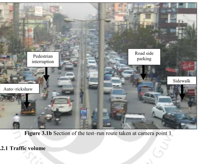
- Traffic volume 41
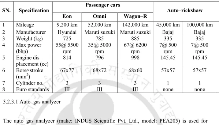
- Test vehicles 42
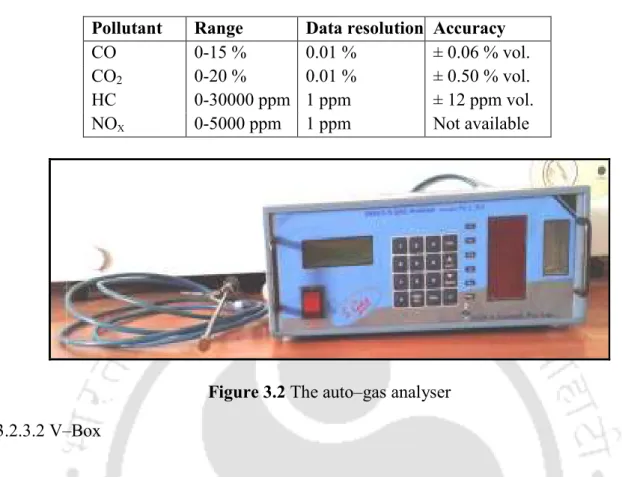
- Instrumentations 42
- Instantaneous tail–pipe emission and speed 44
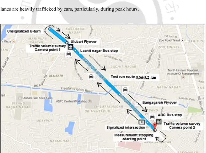
Fieldwork was carried out to collect data on traffic volume, data on current tailpipe emissions of test vehicles (passenger cars and auto-rickshaws) and vehicle speed. The V–Box measures the current speed, position of the vehicle and records data with a data recording frequency of 10 Hz (Figure 3.3). Current emissions and speed measurements were carried out in both directions of the test track by integrating the autogas analyzer and V-Box with computer and camera.
SYNCHRONIZATION OF DATA 47
DATA INPUTS FOR ANALYSIS 48
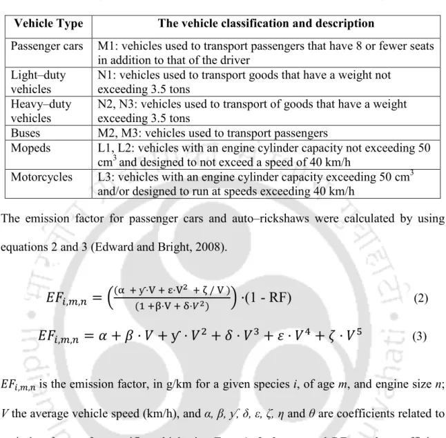
The emission factor for passenger cars and auto-rickshaws was calculated using Equations 2 and 3 (Edward and Bright, 2008). The regression coefficients and R2 values for passenger car and auto-rickshaw are tabulated in Tables 6.5 and 6.6 respectively. The local traffic flow management can reduce the significant level of emissions from petrol passenger cars and auto-rickshaws.
DATA ANALYSIS AND INTERPRETATION 51-64
Traffic–flow rate 51
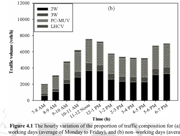
The lowest traffic was observed during 7–8 am. in both cases and higher traffic during 10 a.m.–12 noon and 4–7 p.m., on working days, while on non-working days during 11 a.m. to 1 p.m. 6-7 p.m. The analysis shows that there is a slight difference in the average value of traffic volume for working and non-working days, while the average value of the hourly traffic speed is approximately the same. Table: 4.1 Descriptive statistics for hourly traffic composition and traffic fleet speed for working and non-working days.
Traffic composition 55
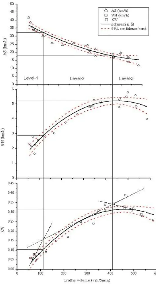
Traffic–flow vs speed 56
Traffic flow mode 2: shows a sharp increase in CV and VN with increasing traffic volume and decreasing traffic speed. Traffic Flow State 3: As traffic volume approaches near lane capacity, CV and VN decrease sharply, forcing vehicles to crawl.
Traffic–flow patterns 57
Instantaneous traffic speed 60
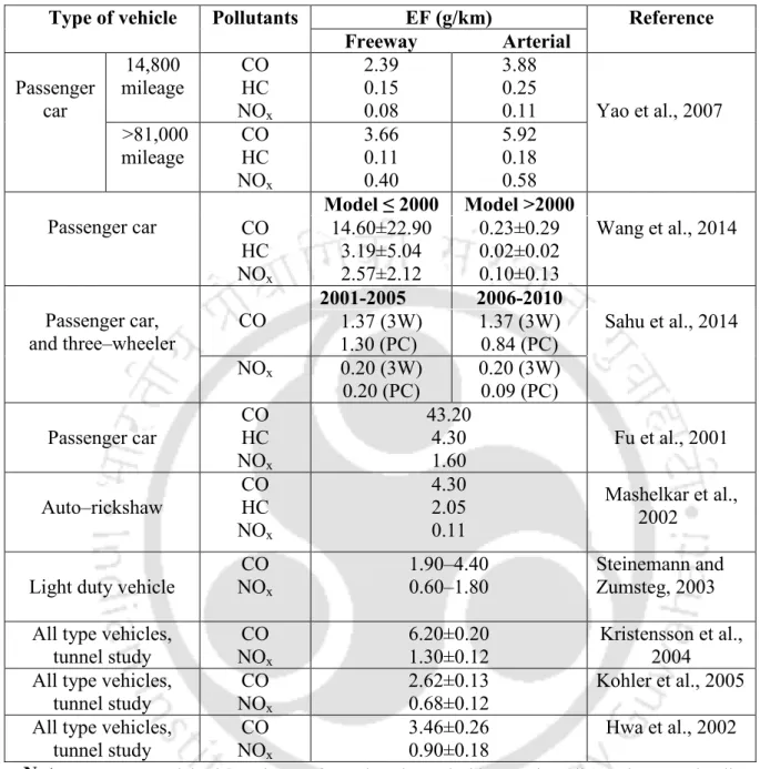
The share of VSP bodies and emission rate of CO, HC, CO2 and NOx for passenger cars and auto rickshaw are shown in Figure 5.8a and 5.8b. The measured emission of CO, HC, CO2 and NOx were compared with the modeled EFs for the passenger car and auto-rickshaw. The instantaneous emissions for this speed of passenger car (mileage 142,000 km/h) and auto-rickshaw (100,000 km/h) were used for analysis.
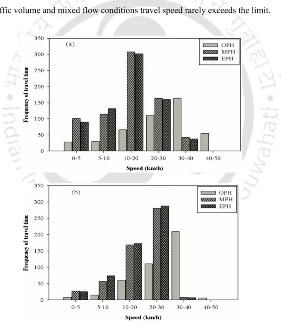
Frequency distribution of travel time and speed 62
INSTANTANEOUS EMISSION ANALYSIS 63
SUMMARY AND DISCUSSION 63
URBAN TRAFFIC EMISSIONS 65-98
INSTANTANEOUS EMISSION 68
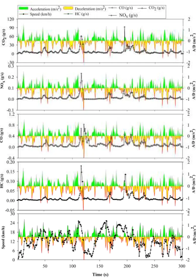
It was found that 70% of the time the test vehicle had a speed of about 30 km/h with several stops and starts. Frequent stop-and-go was found to result in higher peaks in CO, HC and NOx emissions. The stop-and-go pattern includes frequent shifting and high power interval (Elmi and Al Rifai, 2012) and the main causes of higher emissions and thus increases the amount of emissions during PH.
EMISSION FACTORS BY TAIL–PIPE MEASUREMENTS 72
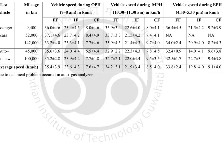
For autorickshaw, the measured EF of CO and HC was found to be about 2–8 times higher under CF and 2–5 times under IF compared to FF condition, and NOx was 2–5 times higher under FF compared to CF. Under PH, the EF for CO and HC was 2–4 times higher compared to OPH and for NOx was about 2 times higher under OPH. Under PH, the EF of CO and HC was found to be about 4–7 times higher from OPH and of NOx was about 2 times higher in OPH.
EMISSION FACTORS BY MODELS 76
- COPERT–IV 76
- IVE 86
It was found that for the passenger car with lower mileage (9200 km), the deviation between measured and modeled EF was smaller. Figure 5.6 (a, b and c) and 5.7 (a and b) show the comparison of measured and modeled EF after mileage correction factors. Therefore, at lower speeds, the measured EF was found to be higher compared to the modeled EF.
COMPARISON OF MEASURED AND MODELLED EF 92
COMPARISON OF COPERT–IV AND IVE MODEL 95
SUMMARY AND DISCUSSION 95
The measured emission factors were further compared with an average velocity model COPERT-IV and instantaneous velocity model IVE. Therefore, this results in a larger deviation in the measured and modeled values compared to IVE. It was found that at lower speeds the measured EFs deviated from the modeled COPERT-IV EF for HC and CO.
IMPACTS ON EMISSIONS AND MITIGATIONS 99-124
TRAVEL TIME AND SPEED VS EMISSION 103
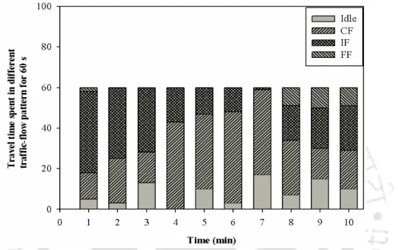
Therefore, the relationship between exhaust gas emissions under different traffic and flow conditions corresponding to a travel time under these conditions of 60 s was analyzed for a period of 10 minutes of test runs. To determine the combined effect of travel time and associated speed on exhaust emissions, a speed-time factor was used, which is the multiplication of the average speed of a given flow class and the time spent for that class. Figures 6.5a and 6.5b show the relationship between the pollutant emission rate and the speed/time factor for a passenger car and an auto-rickshaw, respectively.
MILEAGE VS EMISSION 109
Similarly, for auto-rickshaw, increasing mileage has a significant impact on CO and HC emissions. Summary of the mean emission values obtained from ANOVA for each mileage class is given in Table 6.2, which leads to the conclusion that there is a statistically significant correlation of CO, CO2 and HC emissions with mileage.
UPGRADATION OF EMISSION STANDARDS AND SWITCHING TO
2011b) reported that phasing out conventional two-stroke engine technology appears to be a desirable policy for CNG auto-rickshaws in Delhi. It has been found that with the CNG conversion of the auto-rickshaw, the reduction of 87-89%. Guwahati has a higher percentage of auto-rickshaw travel per day, of which 70% are two-stroke, highly polluting.
TRAFFIC–FLOW MANAGEMENT 115
- Management of public transport 115
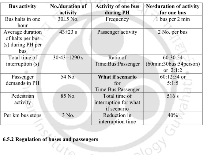
- Regulation of buses and passengers 116
- Comparison of emission reduction strategies 122
- Improvement of traffic–flow 122
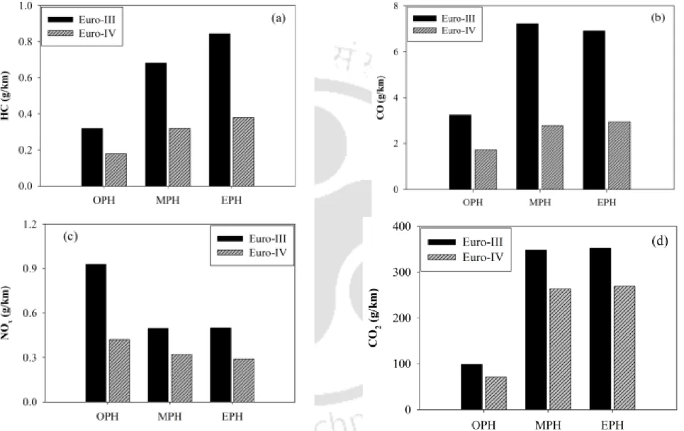
Similarly, the Figure 6.9 (a, b, c and d) shows the emission reduction of auto-rickshaw due to 40% reduction in bus stop time during PHs for pollutants HC, CO, NOx and CO2 respectively. The emission rates of NOx and CO2 at low speed (12±5 km/h and 22±3.5 km/h for passenger car and auto-rickshaw, respectively) were less. The number of bus stops was found to be positively correlated with the HC and CO emissions for both passenger cars and auto rickshaws.
SUMMARY AND DISCUSSION 123
Further, mitigation options related to technology, fuel and traffic flow management were investigated to reduce disruption and associated emissions. Although, an effective public transport system consisting of buses is a good solution and has been used in many countries around the world (Koshy and Arasan, 2005; . Tang et al., 2009), in Indian traffic conditions, the lack of respecting the lanes. , chaotic bus stops on urban roads often cause disruptions and traffic jams. Therefore, the traffic management strategy as studied in this research can reduce interruptions and congestion and the associated higher emissions.
GENERAL CONCLUSION . 125
SPECIFIC CONCLUSION 125
The extent of emission is the combination effect of higher frequency of travel time and low speed, especially for the pollutants CO and HC, while the emission of NOx increases with the increasing speed. The peak hour emissions are drastically reduced for the technology switch and the use of cleaner fuel type (CNG), i.e. switching to cleaner auto-rickshaw fuel has up to 89% reduction in HC and CO, 23–56% in NOx and 32–36% reduction in CO2 emissions.
SPECIFIC FINDINGS OF THE RESEARCH 127
CONTRIBUTION OF THE RESEARCH 127
The classification of different traffic flow patterns (free flow, interrupted flow and congested flow) based on the operating speeds was done. The actual on-road emission factors of different kilometers of test vehicles for different traffic flow patterns were found out. The causes of frequent disruption and congestion on a road busy with urban traffic have been identified as unregulated bus stops and poor pedestrian infrastructure.
LIMITATION OF THE RESEARCH 128
The findings of this research were used to demonstrate how emissions from urban transport can be reduced by implementing various measures (upgrading to higher emission standards, switching to cleaner fuels and regulating city bus frequency).
FUTURE SCOPE 128
Vehicle emissions and level of service standards:. exploratory analysis of the effects of traffic flow on vehicle greenhouse gas emissions. The causes and consequences of particulate air pollution in urban India: a synthesis of the science. A Study of the Causes, Consequences and Improved Measures of Road Traffic Congestion in Lagos Metropolis.