List of Symbols
H Height of water on the upper side of the dam y Change in distance in the vertical direction. ET Tangent Young's modulus for material Duncan-Chang Eur Young's modulus for unloading and reloading.
CONTENTS
HYDRODYNAMIC PRESSURE OF THE RESERVOIR 80
INTRODUCTION
- GENERAL
- IMPORTANCE OF SOIL-STRUCTURE INTERACTION EFFECT
- COMPONENTS OF SOIL-STRUCTURE INTERACTION
- Modeling of Structure
- Modeling of Soil
- Modeling of Radiation Boundary Condition
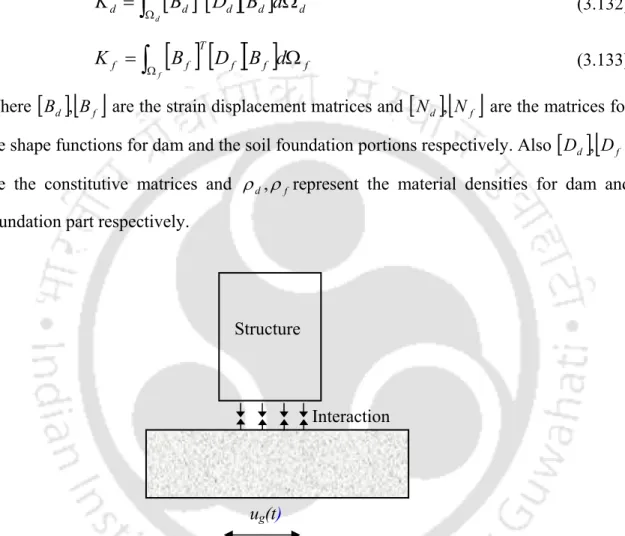
- Modeling of Coupled Dam-Foundation System
- OBJECTIVE OF THE STUDY
- ORGANIZATION OF THE REPORT
For the structure on the rigid foundation, the horizontal movement can be applied directly to the base of the structure. For a given steering motion, the seismic response of the structure depends only on the properties of the structure.
REVIEW OF LITERATURE
INTRODUCTION
TRADINATIONAL ANALYSIS OF DAM
- Traditional Static Analysis and Design
- Linear Dynamic Analysis of Dam
- Nonlinear Dynamic Analysis of Dam
When flexibility of dam is considered, the hydrodynamic responses show high peaks at the natural frequencies of the system (Saini et al. 1978). The mass matrix of the structure. u} = The vector of nodal point displacements relative to ground.
HYDRODYNAMIC PRESSURE ON DAMS
The response of the dam did not contribute to the interaction forces because it was assumed to be rigid. He found that the response of the dam increases significantly if the fluid-structure interaction is taken into account.
CONCRETE DEGRADATION
Lindvall (2001) has determined the mathematical relationship of the service life of concrete structures, which depends on material properties, the construction process and the environmental effects. -Silica Reaction (ASR) approach to determine the degradation of the concrete structures was proposed by Steffens et al.
MODELING OF FOUNDATION
- Material Nonlinearity
- Integration of Nonlinear Constitutive Equations
A detailed description of all the different types of models used in the numerical simulation of soil behavior is. In non-associated plasticity, the system of equations of the tangential stiffness method is non-symmetric.
INTERACTION AND RADIATION CONDITION
- Numerical Methods to Tackle Radiation Condition .1 Finite Element Method
But these absorbing boundary conditions had much less impact in the context of the finite element method. Wolf and Song (1996) developed the scaled boundary element method (also known as consistent infinitesimal finite element cell method) by combining the advantages of the boundary element method and the finite element method.

SOIL STRUCTURE INTERACTION ANALYSIS
- Static Soil-Structure Interaction Problems
- Dynamic Soil-Structure Interaction Problems .1 Linear Analysis
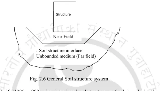
A consistent free-field ground motion was applied to the boundaries of the discrete model and the response of the combined soil structure system was calculated. Determination of the response of the unconfined soil at the general soil-structure interface in the form of a displacement-force relationship. An example application of the staggered approach in the context of soil structure interaction analysis is that of Rizos and Wang (2002).
The majority of work done worldwide in soil structural analysis is limited to linear analysis. The results of tests of the soil structure system model have been presented, which are in good agreement with those obtained by analysis using the proposed model.
SUMMARY OF THE LITERATURE
An efficient coupling procedure was formulated that involves applying the boundary condition of Sharan (1987) at the far end of the infinite fluid domain. The aging process of concrete is a very important phenomenon which leads to the loss of rigidity of the concrete structure. In most cases, soil-structure interaction analysis is performed considering the foundation material to be linear, elastic.
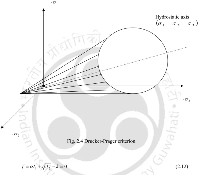
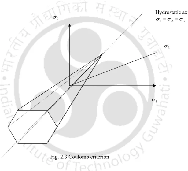
Therefore, to truly assess the behavior of the soil-structure system during interaction analyses, the nonlinear material properties of the foundation should be considered. The Von-Mises, Tresca, Mohr-Coulomb and Drucker-Prager models make up the bulk of the elastoplastic models available for geomaterials.
SCOPE OF THE PRESENT INVESTIGATION
THEORETICAL FORMULATION
INTRODUCTION
But the actual stress-strain behavior of the soil/rock material is essentially non-linear. In order to truly represent the actual behavior of the soil/rock foundation material, a non-linear constitutive model should be considered. A number of methods are available to represent the nonlinear stress-strain behavior of soil/rock material.
The coupled effects of the dam-foundation system are obtained by introducing an iterative scheme that simulates the interaction behavior. Parts A, B and C contain the formulations of the aged dam, foundation and the connected dam foundation system respectively.
SUITABILITY OF FINITE ELEMENT TECHNIQUE
- Selection of Finite Element
- Shape Functions
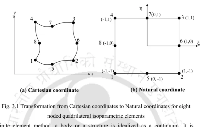
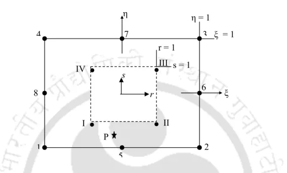
- Re lationship Between Cartesian and Natural Coordinates The displacements u and v are expressed using the interpolation functions as
Similar to the absorbing boundary condition, a combination of springs and dashpots can be used to absorb the energy of the incoming waves. Due to complex geometry of the embankment foundation system, a straightforward analytical solution may not be achievable. The eight-noded quadratic isoparametric finite element is one of the most versatile and efficient elements used to model irregular domain geometries.
Natural coordinates are always associated with an element and are scaled so that the sides of the parent element are defined by ξ = ±1 and η = ±1. An eight-node quadrilateral element as shown in Figure 3.1 is considered to discretize the dam and foundation domain.
TIME DOMAIN SOLUTION OF DYNAMIC EQUATION OF MOTION
- Stability Analysis of Newmark Method
- Accuracy Analysis of Newmark’s method
Stability is achieved if the chosen time step is small enough to accurately integrate the response in the highest frequency component. In practical analysis, the choice of the integration operator depends on the cost of the solution, which can be determined by the number of time steps required for the integration. For a conditionally stable algorithm such as central difference, the time steps for a given. the time range considered is determined by the critical time step Δtcr and there are not many choices available.
Damping does not affect stability if the 2nd γ allowable time step is increased by damping. When the ratio of time step to period is larger, different integration methods have quite different characteristics.
PART A
THEORETICAL FORMULATION FOR DAM
- Strain Displacement Relationships
- Constitutive Matrix
- Degradation Model for Concrete
- Evaluation of Degradation Index
The concept of concrete strength degradation is based on the reduction of the net surface that can withstand stresses. In general, the description of the deterioration of concrete structures by ASR includes two basic aspects: the kinetics of the chemical reactions involved, which lead to the formation of the product of the expansive reaction, i.e. of the swollen gel, and the mechanical damage caused by this formation. A detailed description of gel formation and other mechanisms is well described in the work of Steffens et al.
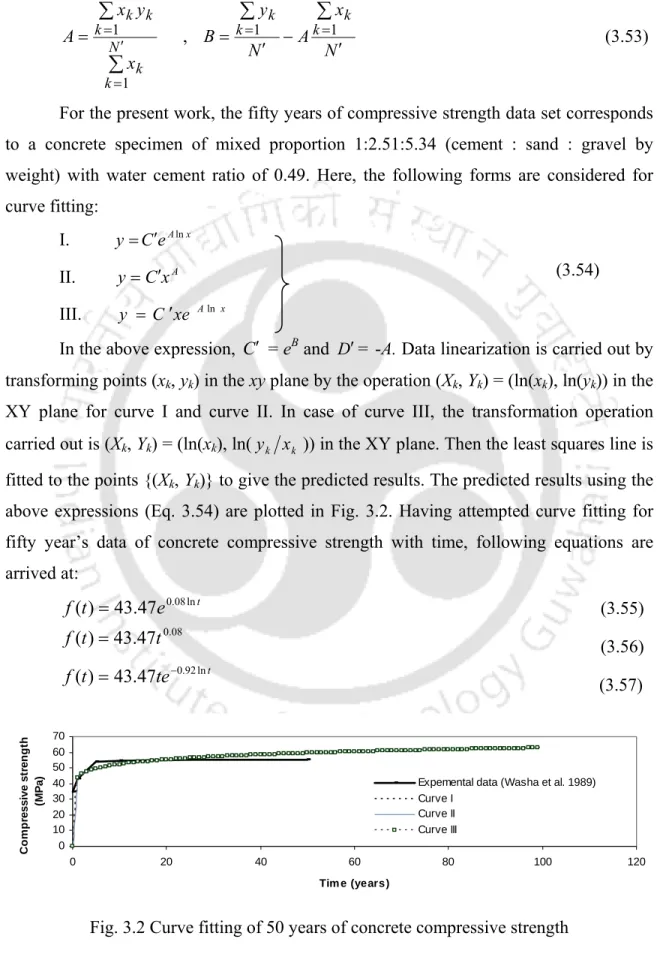
Equation (3.56) was obtained by performing a least-squares analysis using a curve of the form y=C′xA with the necessary transformation of the coordinates as previously mentioned. Equation (3.57) was obtained by performing a least-squares analysis by performing a curve of the form y=C′xeAlnx with the necessary transformation of the coordinates as previously mentioned.
STIFFNESS, MASS AND DAMPING MATRICES
Equation (3.55) was obtained by least squares analysis using a curve of the form y=C′eAlnx with the necessary coordinate transformation as mentioned earlier. 3.2, it can be observed that the results obtained from Eq. 3.57) are all similar and these results agree quite well with the experimental data. In this analysis, Equation 3.56) was used to predict the strength gain of concrete with aging.
The value of static elastic modulus of concrete in SI units (Neville and Brooks, 1987) is obtained from. Including the effect of point charges{ }p i, Eq. 3.62) can be expressed in matrix form as follows.
Computation of Stresses
Unfortunately, when determining the voltages at the junctions, it turned out that they are discontinuous in nature. Attempts to calculate stresses directly at the nodes have proven to be very poor sampling points (Zienkiewicz and Taylor 1991), although the nodes are the most useful points for voltage output and interpretation. However, it has been observed that shape function derivatives (and thus stresses) evaluated at the inside of the element are more accurate than those calculated at the element boundary.
Hinton and Campbell (1974) have shown how to extrapolate stresses obtained at the Gauss points to the nodes using the "smoothing technique". Hereσ1, σ2…….,σ8 are the smoothed nodal values and σI…σIV are the stresses at the Gaussian points.
HYDRODYNAMIC PRESSURE OF THE RESERVOIR
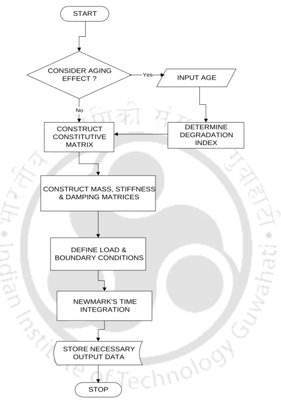
FLOWCHART FOR THE DAM ANALYZER
PART B
THEORETICAL FORMULATION FOR FOUNDATION
- Governing Differential Equation for Foundation Domain
- Constitutive Property for Soil/Rock Material
- Nonlinear Solution Algorithm
In most early investigations into soil-structure interaction phenomena, it is assumed that the stress-strain response of the soil mass is linear, especially because the solution is then obtained in a single step. In this study, an attempt has been made to calculate the actual nonlinear soil behavior obtained from triaxial test data. Because of the generality of the hyperbolic model and its ability to represent the stress-strain behavior of soils ranging from clay and silt through sand, gravel, and rock fill, it can be used for partially saturated or fully saturated soils, as well as for drained or undrained soils. loading conditions in compacted soil materials or natural soils (Duncan, 1980).
However, for this analysis, only the Young's modulus of the rock material is varied according to Eq. Details of the algorithm can be found in Chapter 15 of the book by Chopra (2007).
BOUNDARY CONDITIONS FOR FOUNDATION DOMAIN
- Fixed or Free Boundary
- Absorbing Boundary
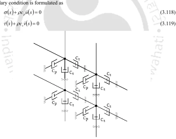
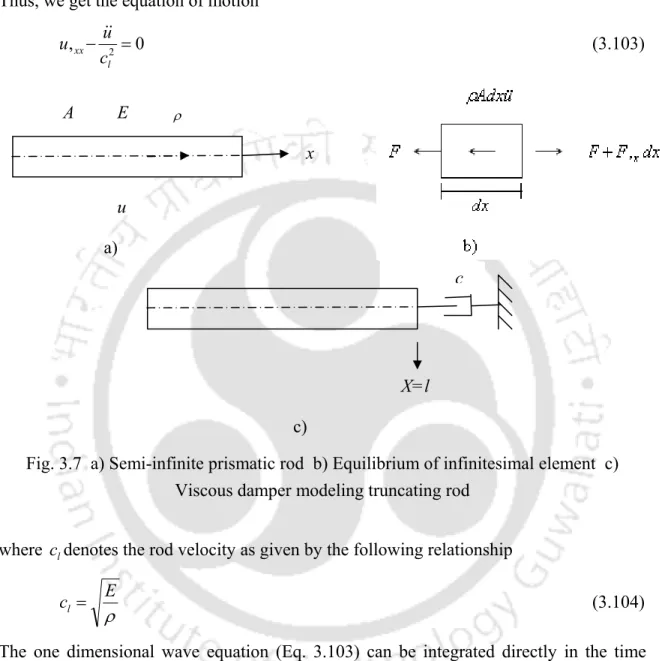
- Viscous Damper for Two Dimensions
- The Effect of earth Pressure
- Finite Element Implementation
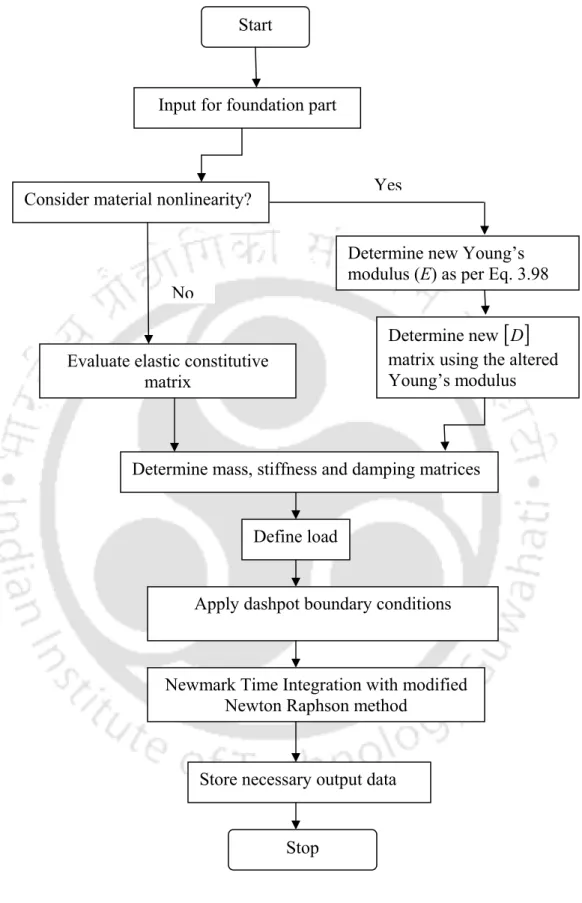
- Flowchart for the foundation analyzer
3.9 (c), the nodes at the base of the boundary are equipped with rollers that only allow horizontal movement. To avoid this, the node in the center of the base is completely fixed in the following analyses. 3.9 (b) and secondly, the boundary nodes at the bottom of the base are fitted with chokes, as shown in Fig.
A detailed description of the use of dashpots can be found in the works by Preisig (2002). The boundary condition at the sides of the foundation boundaries is modified to account for the effect of attached viscosity.
PART C
DAM-FOUNDATION COUPLED SYSTEM
- Iterative Scheme
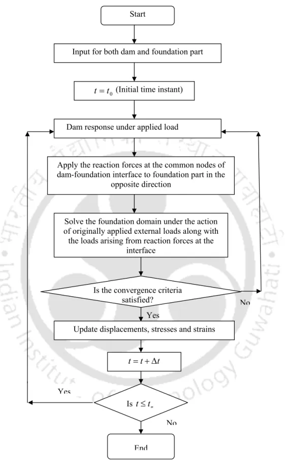
- Flowchart of the Iterative Scheme
The forces exerted give rise to reaction forces at the common nodes in the interface between the dam and foundation. The reaction forces generated at the common interface nodes of structure and foundation are then applied in the opposite direction at the common nodes of the foundation system to solve. After settlement of the foundation member against the applied load of ( ff + fif ), the common interface nodes of the foundation member will undergo some displacement.
The modified boundary condition for the structural domain thus simulates the flexibility of the foundation. Apply the reaction forces at the common nodes of the dam-foundation interface to the foundation member i.
NUMERICAL RESULTS AND DISCUSSIONS
INTRODUCTION
PART – I
Analysis of Dam
- Validation of the Algorithm
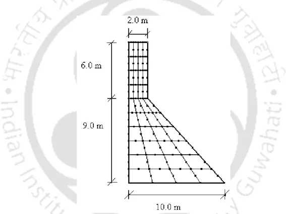
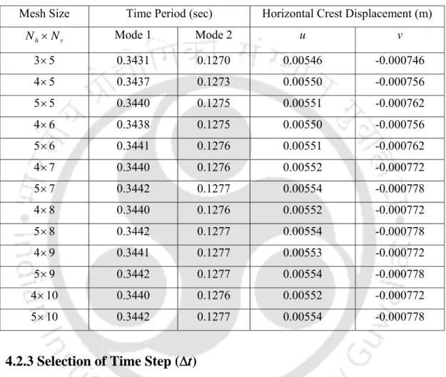
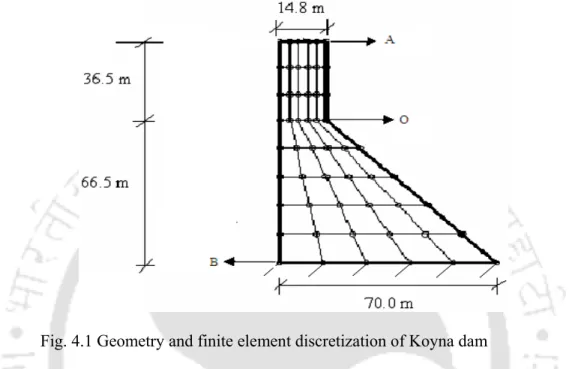
- Discretization of Dam
- Selection of Time Step (Δt)
- Evaluation of Degradation Index
- Response of Aged Dam
- Effect of Hydrodynamic Pressure on Dam
- Summary of Findings
The value of the smallest minor principal stress observed at the immediate end of construction is -6.78 MPa. 4.9, it can be observed that the maximum principal stress occurs at 4.62 sec. just after the construction of the dam. 4.11 (ii) shows the contour plot of the major and minor principal stresses (both σp1 and σp3) throughout the dam at 4.62 sec.
4.12 (ii) plot the distribution of principal and minor principal stresses (both σp1 and σp2) over the entire body of the dam at 4.81 s. 4.9 it can be seen that the maximum value of the principal principal stress occurs at 3.98 s after the 25th year of dam construction.
PART –II
ANALYSIS OF FOUNDATION
- Material Properties of Foundation
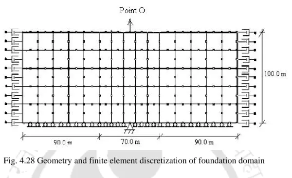
- Discretization of Foundation Domain
- Selection of Time Step (Δt)
- Selection of Foundation Size without Dashpot
- Selection of Foundation Size with Dashpot
- Effect of Foundation Nonlinearity
- Summary of Findings
The dash points are then attached to the nodes at the lateral boundary of the foundation domain. It can be observed that there is a concentration of tensile stresses along the left side of the foundation field. It can be seen that the compressive stresses are dominant along the right side of the foundation.
4.39, it can be seen that the tensile stress occurs along the right side of the foundation. The left-center section at the base of the foundation also experiences concentration of tensile stresses.
ANALYSIS OF DAM-FOUNDATION COUPLED SYSTEM
- Validation of the Proposed Iterative Scheme
- Response of Dam-Foundation Coupled System
- Parametric Studies for Dam-Foundation Interaction Analyses under Full Reservoir Condition
4.51 (ii) shows that the maximum compressive stress occurs near the heel part of the dam body. 4.59 (ii) shows that compressive stresses are generated near the neck region of the dam body. 4.61 (ii) shows that compressive stresses are generated near the neck region of the dam body.
4.66 (ii) shows that the compressive stress is concentrated near the neck region of the dam body. 4.68 (ii) shows that the compressive stress is concentrated near the neck region of the dam body.