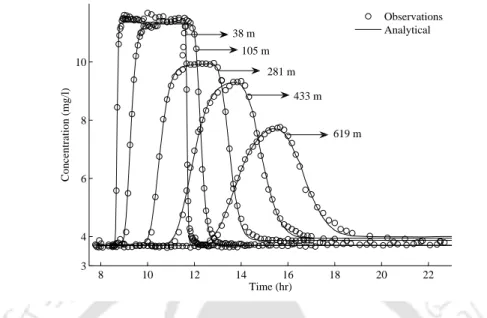
24 2.3 Comparison of concentration profiles of the given analytical solution. 2.17) (solid lines) and observed concentration profiles (open dots) from the Uvas Creek tracer experiment for the TSM. 4.21) (solid lines) and observed concentration profiles (open dots) from the Uvas Creek tracer experiment for the diffusive transfer model.
Introduction
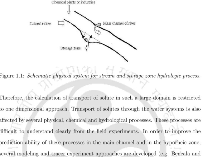
Due to the slow release of the solute particles from the storage zone into the main channel of the stream, it becomes. Storage zone is a stagnant water zone that is stagnant relative to the main flow of the stream.
Transient storage models due to first order mass exchange
They considered the lateral inflow as distributed inflow and estimated the parameters of the TSM. 11] evaluated the parameters of the TSM for the five tracer experiments conducted in the Chill´an River, Chile.
Transient storage models due to diffusive exchange
The processes of advection and dispersion in flows are described by the one-dimensional advection-dispersion equation in the main flow channel. The advection-dispersion equation in the main flow channel is related to the diffusive exchange term.
Objectives
In the second problem we derive analytical solutions from the RSTM with decay, sorption and lateral inflow. The analytical solution for the main channel is compared to the observed data from the Uvas Creek tracer experiment for conservative (chlorine) solute.
Governing equations
- Assumptions for the model
- General boundary and initial conditions
- Dimensionless forms of governing equations, general boundary
- Calculation of the cross-sectional average velocity (u ? m )
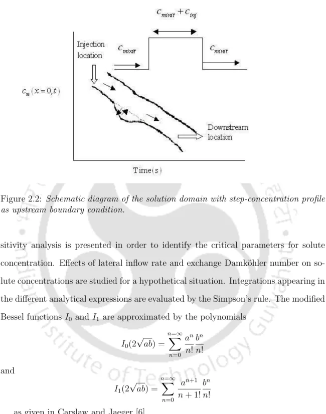
So the upstream boundary condition can be expressed as. 2.3) where x?0 is the upstream boundary location and c?u(t?) is the upstream concentration at the location x?0 and time t?. The dimensionless forms of the governing equations, general boundary and initial conditions given in are written as. 0) is the concentration in the main channel of the river, c?0 is the plateau concentration at the head of the tracer experiment, cs(= cc?s?.
Analytical solution for conservative solutes with storage zone
The analytical solution for the storage area is obtained by substituting Eq. 2.14) and with the inverse Laplace transform we get It is easy to see that the analytical solution presented in Eq. 2.17) reduces to the analytical solution of the classical advection-dispersion equation with lateral inflow when Daem = 0 (i.e., there is no mass exchange between the storage zone and the main channel).
Results and Discussion
Application to tracer experiment
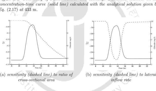
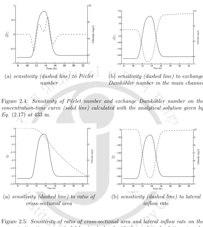
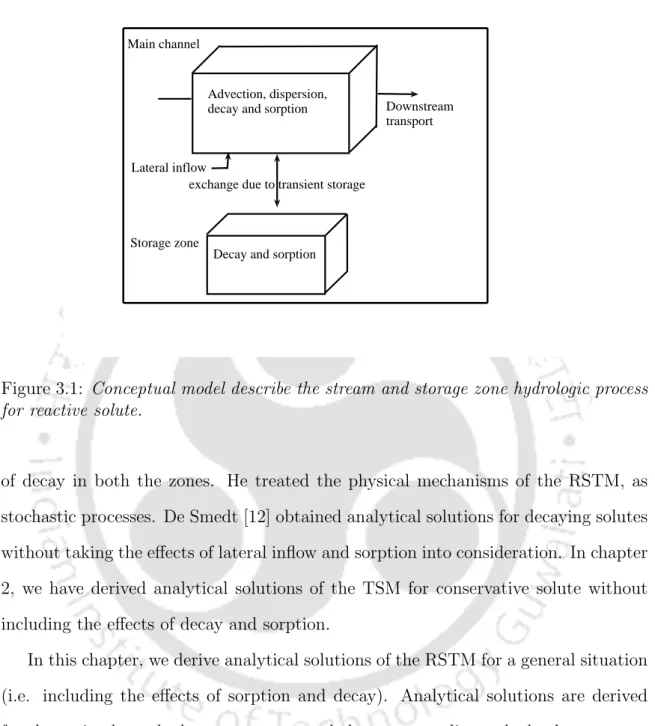
The estimated value of lateral inflow (q?L) increases gradually with slight oscillation and the average volumetric flow rate (Q?) also increases downstream, as shown in Table 2.1. Values of the parameters also follow the same trend as presented in the work of Bencala and Walters [2]. Sensitivity is the partial derivative of the simulated flow tracer concentration with respect to a change in the value of a parameter (Wagner and Harvey [39]).
Hypothetical Experiment
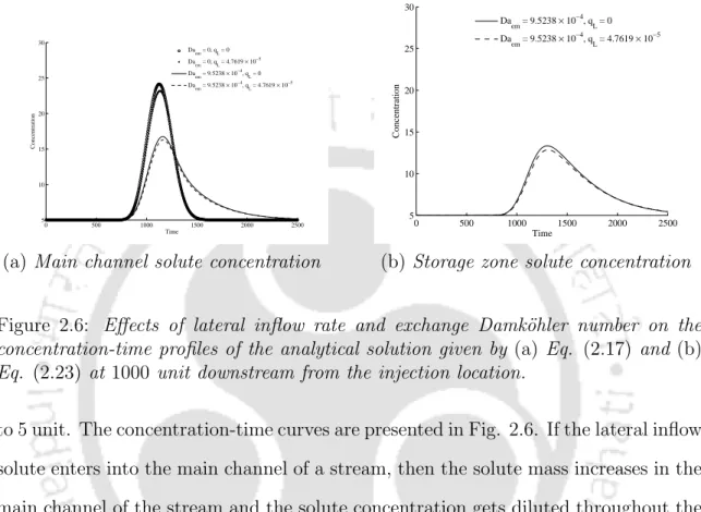
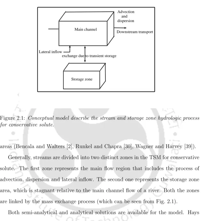
It reveals that the concentration change in the main channel is the largest due to the exchange of solute between the main channel and the storage area. a) sensitivity (dashed line) to the P´eclet number. If a side inflow solute enters the main stream channel, the mass of the solute increases in the main stream channel and the solute concentration is diluted throughout the study reach compared to the case without side inflow. This mass exchange is the main cause of the solute mass reduction and also forms a long tail at the lower edge of the solute concentration profiles in the main channel at the downstream location compared to the case where there is no storage area.
Conclusions
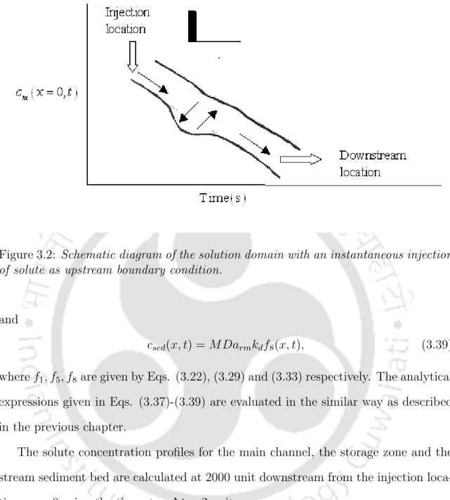
First-order reaction and decay are considered in the main channel as well as in the storage zone. The transient storage model (TSM) of Bencala and Waters [2] was extended by Bencala [3] for the reactive solute by including absorption effects in the main channel as well as in the storage zone. The first model deals with breakdown in the main channel as well as transient deposition (De Smedt [12], Schmid [33]), while the second deals with absorption in the bed sediments of lateral streams [3].
Governing equations
Assumptions for the model
ˆλ?m(kdc?m−c?sed), (3.3) where c?m is the solute concentration in the main direction of current flow, c?s is the solute concentration in the deposition zone, ˆc? s is the equilibrium solute concentration in the deposition area, c?sed is the sorbate concentration in the streambed sediment, c?L is the solute concentration at the lateral inlet, u?m is the mean cross-sectional velocity at the main channel, x. is time, D?m is the longitudinal dispersion coefficient in the main stream, A?m is the cross-sectional area of the main stream channel, A?s is the cross-sectional area of the deposition area, α. is the rate at which mass is exchanged from the main channel to the storage area, qL. is the rate of lateral entry into the stream per unit length of the stream, ρ is the mass of accessible sediment per volume of stream water, ˆλ?m is the first-order absorption rate coefficient in the main channel, kd is the distribution coefficient , ˆλ?s is the first-order absorption rate coefficient in the storage area, λ?m is the first-order decay coefficient in the main channel, and λ?s is the first-order decay coefficient in the storage area. 3.1) and (3.2) of this study are obtained by adding the terms for the first-order mass transfer reaction and also for the first-order decay in the main channel as well as in the deposition zone in Eqs. 2.1) and (2.2) of the transient storage model (TSM) for the conservative solute (described in chapter 2). 3.3) shows that the rate of change of the concentration of the absorbing element in the bed sediment is proportional to the difference between the solute concentration in the stream bed sediment and its potential equilibrium concentration in the main channel.
General boundary and initial conditions
Dimensionless forms of governing equations, general boundary
Analytical solution for kinetic transport of reactive solutes with storage
With the help of convolution theorem (given in Prudnikov et al. [27], Sneddon [36]), inverse Laplace transform of Eq. The analytical solution for the storage zone is obtained by Eq. 3.17) and applying inverse Laplace transform as, . The analytical solution for the stream sediment bed is also obtained by Eq. 3.18) and applying inverse Laplace transform as, .
Results and Discussion
Hypothetical Experiment
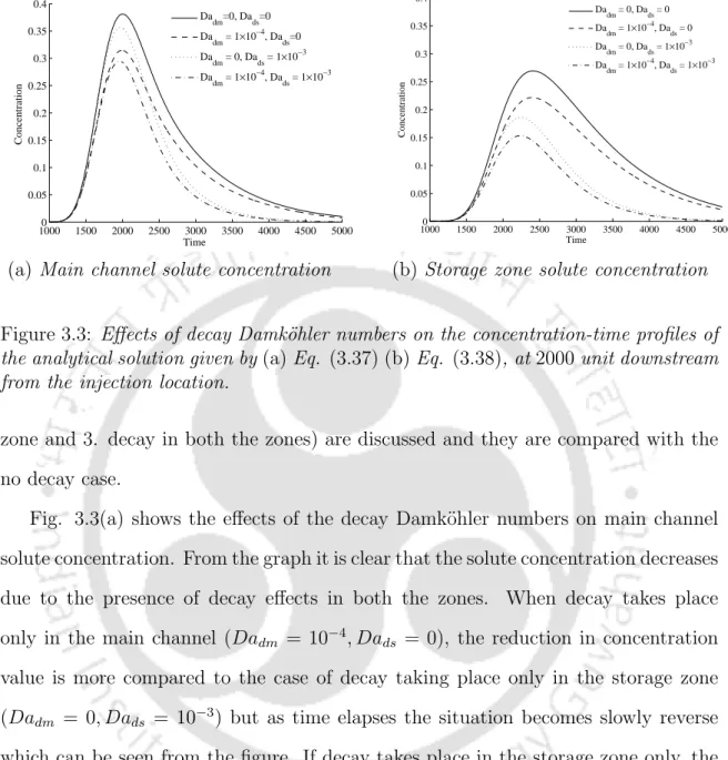
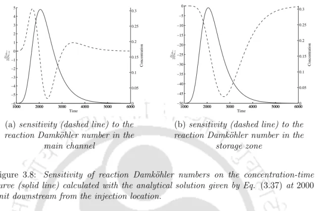
Solute concentrations in the main channel, in the storage area, and in the stream sediment bed were calculated. It is observed that the concentration-time curves show similar effects of Dars in the main channel and its sedimentary bed. A sensitivity analysis is performed for the parameters: decay Damk¨ohler number in the main channel (Dadm), decay Damk¨ohler number in the storage area (Dads), reaction Damk¨ohler number in the main channel (Darm) and reaction Damk¨ohler number.
Conclusions
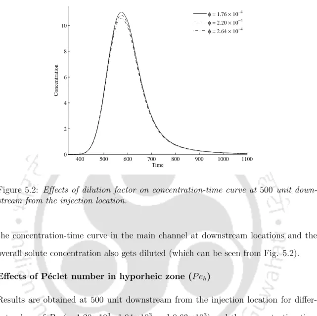
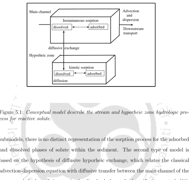
This chapter deals with the derivation of analytical solutions for solute transport in a flow in the presence of hyporheic zone, where solute exchange between the main channel and hyporheic zone is dominated by the diffusive exchange. De Smedt [13] presented an analytical solution of the model in the case of instantaneous injection of conservative solute for constant and uniform flow. A hypothetical situation is considered to study the effects of dilution factor, P´eclet number and porosity in the hyporheic zone on the breakthrough curves.
Governing equations
Assumptions for the model
Advection does not occur in the hyporheic zone and only diffusion affects the solute concentration in this zone. The solute concentration in liquid water can only change in the longitudinal direction, while the solute concentration in the hyporheic zone can change in both the longitudinal and transverse directions. The solute exchange between the main channel and the hyporheic zone is represented by the term diffusive exchange.
General boundary and initial conditions
4.1) is obtained by relating the classical one-dimensional advection-dispersion equation to a diffusive exchange between the main stream channel and the hyporheic zone.
Dimensionless forms of governing equations, general boundary
It is easy to see that Eq. 4.9), in the absence of the dilution factor, the classical advection-dispersion equation becomes when P eh → ∞ (i.e. the tracer particles do not enter the hyporheic zone).
Analytical solution for diffusive transfer of conservative solutes with
With the help of convolution theorem (given in Prudnikov et al. [27], Sneddon [36]), inverse Laplace transform of Eq. 4.27). The analytical solution for the hyporheic zone solute concentration is obtained by Eq. 4.18) and applying inverse Laplace transform as, .
Results and Discussion
Application to tracer experiment
On the other hand, Figure 4.2 shows that the diffusion transfer model is free from the above disadvantages of TSM and gives more accurate results. A sensitivity analysis is performed to define the sensitivity of the diffusive transfer model parameters. The results for the sensitivity of the solute concentration to various parameters are presented in fig.
Hypothetical Experiment
The increase in the dilution factor is the main cause of the reduction in the mass of the solute in the main channel at downstream locations. a) sensitivity (dashed line) to the P´eclet number in the main channel. It shows that as the value of P eh decreases, the concentration-time curve becomes more asymmetric. To study the effects of porosity (²) on the concentration-time curves in the main flow channel, different values of ² were chosen and the results are shown in Fig.
Conclusions
The second type of model is based on the hypothesis of diffuse hyporheic exchange, which relates the classical advection-dispersion equation to diffuse transfer between the main channel of the flow and the hyporheic zone in the dissolved phase of the solute (Jackman et al. [21) . ], W¨orman [40]). 23] took into account the dispersion in the main channel and the kinetic response due to sorption in both zones. A hypothetical situation is considered to study the effects of dilution factor (φ), P´eclet number (P eh), porosity (²), sorption Damk¨ohler number (Dash) and equilibrium partition coefficient (kh) on the concentration. -time curves in the main channel.
Governing equations
Assumptions for the model
In the stream water, the sorption on the particles immediately reaches equilibrium, and the sorption in the hyporheic zone is described as a first-order kinetic reaction. 5.2) represents the one-dimensional diffusion equation for the dissolved solute concentration in the hyporheic zone with a first-order kinetic reaction between the adsorbed and dissolved solute concentrations. 5.3) represents a first-order linear relationship between the adsorbed and dissolved phases of the solute concentration in the hyporheic zone.
General boundary and initial conditions
5.1) is obtained by connecting the one-dimensional classical advection-dispersion equation for the main channel with the diffusion exchange between the main flow channel and the hyporheic zone. 5.3) represents a first-order linear relationship between the adsorbed and dissolved phases of the solute concentration in the hyporheic zone. 5.10) where c?minit(x?), c?hdinit(x?, z?) and c?hainit(x?, z?) are the initial concentrations of the solute in the main channel, in the dissolved and adsorbed phase of the hyporheic zone or
Dimensionless forms of governing equations, general boundary
5.10) where c?minit(x?), c?hdinit(x?, z?) and c?hainit(x?, z?) are the initial concentrations of the solute in the main channel, in the dissolved and adsorbed phases of hyporhea. area respectively.
Analytical solution for diffusive diffusive transfer of reactive solutes
With the help of the convolution theorem (given in Prudnikov et al. [27], Sneddon [36]), the inverse Laplace transform of Eq. 5.33). The analytical solution for the solute concentration in the hyporheic zone is obtained by substituting Eq. 5.23) and applying the inverse Laplace transform as,.
Results and Discussion
Hypothetical Experiment
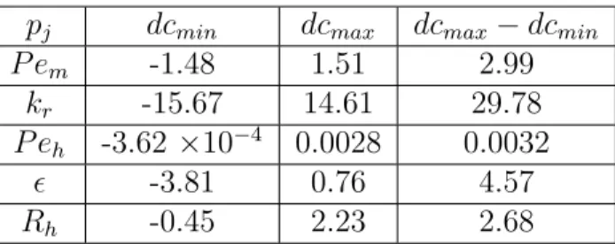
It shows that the peak value of the concentration-time curve decreases as the value of ² increases. Effects of sorption Damk¨ohler number and equilibrium distribution coefficient in the hyporheic zone. As the porosity value (²) increases, the solute concentration in the main channel decreases.
Sensitivity analysis shows that the Damköhler number in the main channel (Daem) and the lateral inflow velocity (qL) are much more sensitive compared to the P´eclet number in the main channel (P em) and the ratio of the cross-sectional areas (kr). Sensitivity analysis shows that the Damköhler number in the hyporheic zone is the most sensitive parameter.