Validation of Selection Function, Sample Contamination and Mass Calibration in Galaxy Cluster Samples

Validation of Selection Function, Sample Contamination and Mass Calibration in Galaxy Cluster Samples

S. Grandis,

^1,2?

M. Klein,

^1,3

J. J. Mohr,

^1,2,3

S. Bocquet,

^1,2

M. Paulus,

^1,3

T. M. C. Abbott,

⁴

M. Aguena,

^5,6

S. Allam,

⁷

J. Annis.

⁷

B. A. Benson,

^7,8,9

E. Bertin,

^10,11

S. Bhargava,

¹²

D. Brooks,

¹³

D. L. Burke,

^14,15

A. Carnero Rosell,

¹⁶

M. Carrasco Kind,

^17,18

J. Carretero,

¹⁹

R. Capasso,

²⁰

M. Costanzi,

^21,22

L. N. da Costa,

^23,24

J. De Vicente,

¹⁶

S. Desai,

²⁵

J. P. Dietrich,

¹

P. Doel,

¹³

T. F. Eifler,

^26,27

A. E. Evrard,

^28,29

B. Flaugher,

⁷

P. Fosalba,

^30,31

J. Frieman,

^7,32

J. Garc´ıa-Bellido,

³³

E. Gaztanaga,

^30,31

D. W. Gerdes,

^28,29

D. Gruen,

^34,14,15

R. A. Gruendl,

^17,18

J. Gschwend,

^6,24

G. Gutierrez,

⁷

W. G. Hartley,

^13,35

S. R. Hinton,

³⁶

D. L. Hollowood,

³⁷

K. Honscheid,

^38,39

D. J. James,

⁴⁰

T. Jeltema,

³⁷

K. Kuehn,

^41,42

N. Kuropatkin,

⁷

M. Lima,

^6,7

M. A. G. Maia,

^7,24

J. L. Marshall,

⁴³

P. Melchior,

⁴⁴

F. Menanteau,

^17,18

R. Miquel,

^45,19

R. L. C. Ogando,

^23,24

A. Palmese,

^7,8

F. Paz-Chinch´ on,

^17,18

A. A. Plazas,

⁴⁴

A. K. Romer,

¹²

A. Roodman,

^14,15

E. Sanchez,

¹⁶

A. Saro,

^21,22,46

V. Scarpine,

⁷

M. Schubnell,

²⁹

S. Serrano,

^30,31

E. Sheldon,

⁴⁷

M. Smith,

⁴⁸

A. A. Stark,

⁴⁰

E. Suchyta,

⁴⁹

M. E. C. Swanson,

¹⁸

G. Tarle,

²⁹

D. Thomas,

⁵⁰

D. L. Tucker,

⁷

T. N. Varga,

^3,51

J. Weller,

^3,51

R. Wilkinson

¹²

Accepted XXX. Received YYY; in original form ZZZ

ABSTRACT

We construct and validate the selection function of the MARD-Y3 sample. This sam- ple was selected through optical follow-up of the 2nd ROSAT faint source catalog (2RXS) with Dark Energy Survey year 3 (DES-Y3) data. The selection function is modeled by combining an empirically constructed X-ray selection function with an in- completeness model for the optical follow-up. We validate the joint selection function by testing the consistency of the constraints on the X-ray flux–mass and richness–

mass scaling relation parameters derived from different sources of mass information:

(1) cross-calibration using SPT-SZ clusters, (2) calibration using number counts in X-ray, in optical and in both X-ray and optical while marginalizing over cosmological parameters, and (3) other published analyses. We find that the constraints on the scaling relation from the number counts and SPT-SZ cross-calibration agree, indicat- ing that our modeling of the selection function is adequate. Furthermore, we apply a largely cosmology independent method to validate selection functions via the compu- tation of the probability of finding each cluster in the SPT-SZ sample in the MARD-Y3 sample and vice-versa. This test reveals no clear evidence for MARD-Y3 contamina- tion, SPT-SZ incompleteness or outlier fraction. Finally, we discuss the prospects of the techniques presented here to limit systematic selection effects in future cluster cosmological studies.

Key words: large-scale structure of Universe – X-rays: galaxies: clusters – methods:

statistical – galaxies: clusters: general

? E-mail: s.grandis@physik.lmu.de

©2018 The Authors

arXiv:2002.10834v2 [astro-ph.CO] 26 Feb 2020

1 INTRODUCTION

The number of galaxy clusters as a function of mass and red- shift is generally accepted as being one of the major sources of information on the composition and evolution of the Uni- verse (see, for instance, Haiman et al. 2001; Albrecht et al.

2006; Allen et al. 2011, and references therein). Cluster num- bers can be predicted by multiplying the number density of halos, the ”halo mass function” (HMF), with the volume sampled. The HMF is highly sensitive to the matter density and the amplitude of matter fluctuations and can be accu- rately calibrated by simulations (e.g., Jenkins et al. 2001;

Warren et al. 2006; Tinker et al. 2008; Bocquet et al. 2016;

McClintock et al. 2019b). The cosmological volume is depen- dent on the expansion history. Together with the redshift evolution of the amplitude of fluctuations, this makes the redshift evolution of the number of clusters very sensitive to the yet unexplained late time accelerated expansion of the Universe.

Clusters can be selected in large numbers through their observational signatures at different wavelengths. In X-rays, the intra cluster medium (ICM), heated by having fallen into the cluster’s gravitational potential emits a strong and diffuse thermal emission in X-rays (see Vikhlinin et al. 1998;

B¨ohringer et al. 2001; Romer et al. 2001; Clerc et al. 2014;

Klein et al. 2019, for selections based on this signature).

At optical wavelengths, clusters can be identified as over- densities of red galaxies (for recent applications to wide pho- tometric surveys, see e.g. Koester et al. 2007; Rykoff et al.

2016). In the millimeter regime inverse Compton scatter- ing of the cosmic microwave background (CMB) photons with the ICM makes clusters detectable as extended shad- ows in CMB maps. This phenomenon is called the Sunyaev- Zel’dovich effect (SZE, Sunyaev & Zeldovich 1972). Scan- ning CMB-surveys for such shadows enables the detection of near-complete, approximately mass-limited cluster samples (Hasselfield et al. 2013; Bleem et al. 2015; Planck Collab- oration et al. 2016; Hilton et al. 2018; Huang et al. 2019) .

Inference of the mass distribution, and thereby cosmo- logical constraints, is limited by the ability to characterise in- completeness, contamination, and the observable–mass map- ping in each of these selection techniques. This leads to the problem of determining the selection function of any clus- ter sample. The problem is split into to parts: determining how the selection function depends on the X-ray, optical, or SZE observables, and calibrating the scaling relation be- tween that observable and cluster mass. The latter is called mass calibration (for a review, see Pratt et al. 2019). It is tackled by measuring the cluster gravitational potential ei- ther through the coherent distortion of background galaxies due to weak gravitational lensing (e.g., Bardeau et al. 2007;

Okabe et al. 2010; Hoekstra et al. 2012; Applegate et al.

2014; Israel et al. 2014; Melchior et al. 2015; Okabe & Smith 2016; Melchior et al. 2017; Schrabback et al. 2018; Dietrich et al. 2019; Stern et al. 2019; McClintock et al. 2019a), or the analysis of the projected phase space distribution of mem- ber galaxies whose velocities are measured by spectroscopic observations (Sif´on et al. 2013; Bocquet et al. 2015; Zhang et al. 2017; Capasso et al. 2019a,b). Such techniques are di- rect probes of the clusters’ gravitational potential.

Both X-ray and SZE selections are known to provide

cluster candidate lists with less contamination than those carried out in optical surveys which suffer from projection effects (see for instance Costanzi et al. 2019, and reference therein). In X-ray studies at sufficiently high detection sig- nificance, extent information can be used to control contam- ination (Vikhlinin et al. 1998; Pacaud et al. 2006). Never- theless, optical confirmation is still required to estimate the redshift of the candidates and to reduce the contamination.

Traditionally, targeted imaging of individual cluster candi- dates was performed to this end.

Such campaigns of pointed follow-up have recently been superseded by automated optical confirmation, as for instance by the Multi-wavelength Matched Filter tool (MCMF, Klein et al. 2018). It scans photometric data along the line of sight toward X-ray or SZE cluster candidates with a spatial and color filter to identify cluster galaxies and determine the clusters redshift. Such tools have the ad- vantage of exploiting the ever larger coverage of deep and wide photometric surveys such as the Dark Energy Survey¹ (DES, Dark Energy Survey Collaboration et al. 2016) or the upcoming Euclid Mission²(Laureijs et al. 2011) and the Ru- bin Observatory Legacy Survey of Space and Time³(LSST, Ivezic et al. 2008)) to follow up candidate lists whose size would make pointed observations impractical.

In this work we seek to construct and validate the se- lection function of an X-ray selected and optically cleaned sample. We focus on the MARD-Y3 sample (Klein et al.

2019, hereafter K19) which is constructed by following up the highly contaminated 2nd ROSAT faint source catalog (2RXS, Boller et al. 2016) with the DES data of the first 3 years of observations (between August 2013 and February 2016, DES-Y3, DES Collaboration et al. 2018). Strict opti- cal cuts lead to a final contamination of2.5%at the cost of optical incompleteness, which we model alongside the X-ray selection. The optical follow up also provides measurements of the optical richness of the selected clusters.

First, we confirm the selection function model by con- straining the scalings between X-ray flux and mass, and richness and mass in different ways. We perform a cross- calibration of our observables with the indirect mass infor- mation contained in the SZE-signature of SPT selected clus- ters by cross-matching the two samples to derive the flux and richness scaling relation parameters. Then we constrain the same scaling relations by fitting for the number counts of MARD-Y3 clusters while marginalizing over cosmology. The former method is largely independent of the selection func- tion for the MARD-Y3 sample, while the latter is strongly dependent on it. Consequently, consistent scaling relation parameter constraints from the two methods validate our selection function model.

We also test the selection functions by further devel- oping the formalism of cross-matching and detection prob- abilities introduced by Saro et al. (2015, hereafter S15). We thereby constrain the probability of MARD-Y3 contamina- tion, the SPT-SZ incompleteness and the probability of out- liers from the scaling relations. This also allows us to iden-

1 https://www.darkenergysurvey.org

2 http://sci.esa.int/euclid/42266-summary/

3 https://www.lsst.org/

tify a population of clusters that exhibit either a surprisingly high X-ray flux or surprisingly low SZE-signal.

The paper is organised as follows. In Section 2 presents the conceptual framework within which we model galaxy cluster samples; Section 3 presents the specific validation methods used in this work; and Section 4 contains a de- scription of the MARD-Y3 and the SPT-SZ cluster samples as well as the priors adopted for the analysis. Our main results are presented in Section 5, comprising the different cross-checks on scaling relation parameters that validate our selection function modeling and that enable further checks of the selection functions. The results are then discussed in Sec- tion 6, leading to our conclusions in Section 7. The appen- dices contain more extensive descriptions of the construction and validation of the X-ray observational error model (Ap- pendix A) and a gallery of multi-wavelength images used for visual inspection (Appendix B).

2 CONCEPTUAL FRAMEWORK FOR CLUSTER COSMOLOGY ANALYSES

In the following section we will present in mathematical de- tail the model of the cluster population used in this work to describe the properties of the cluster samples. This discus- sion follows the Bayesian hierarchical framework established by Bocquet et al. (2015). The cluster population is modeled by a forward modeling approach that transforms the differ- ential number of clusters as a function of halo mass M_500c⁴ and redshift z to the space of observed cluster properties, such as the measured X-ray flux fˆ_X, the measured richness λˆ and the measured SZE signal-to-noise ξ. This transfor- mation is performed in two steps. First, scaling relations having intrinsic scatter are utilized to estimate the cluster numbers as a function of intrinsic flux, richness, and SZE signal-to-noise. These relations have several free parameters such as amplitude, mass and redshift trends, intrinsic scat- ter around the mean relation, and correlation coefficients among the intrinsic scatter on different observables. Con- straining these free parameters is the aim of this work, as these constraints characterise the systematic uncertainty in the observable–mass relations. Second, we apply models of the measurement uncertainty to construct the cluster num- ber density as a function of their properties. We also present the modeling of the selection function and of the likelihood used to infer the parameters governing the scaling relations.

2.1 Modeling the cluster population

The starting point of our modeling of the cluster population is their differential number as function of halo mass M_500c and redshiftz, given by

dN dM

_M,z= dn dM _M,z

d²V

dzdΩdzdΩ, (1)

where _dM^dn

_M,z is the halo mass function describing the dif- ferential number density of halos at mass M and redshiftz,

4 M500,c is the mass enclosed in a spherical over density with average density 500 times the critical density of the Universe. For sake of brevity we will refer to M_500,c as M for the rest of this work.

as presented by Tinker et al. (2008); _dzdΩ^d2V dzdΩis the cos- mological volume subtended by the redshift bin dzand the survey angular footprint dΩ.

The mapping from halo mass to intrinsic cluster proper- ties is modeled by scaling relations, which are characterised by a mean relation with free parameters and a correlated scatter. The mean intrinsic relations we use read as hf_Xi= L₀A_X

4πd²_L(z) M h

M_0,X

BX E(z) E(z_0,X)

2 1+z 1+z_0,X

CX

(2) for the X-ray flux⁵,

hλi=A_λ M h

M_0,λ

Bλ E(z) E(z_0,λ)

Cλ

(3) for the richness, and

hζi=A_SZ M h M_0,SZ

BSZ E(z) E(z_0,SZ)

CSZ

(4) for the SZE signal-to-noise in a reference field. h is the present day expansion rate in units of100 km s⁻¹ Mpc⁻¹, andE(z)the ratio between the expansion rate at redshift z and the current day expansion rate. The form of the red- shift evolution adopted in equations (3) and (4) has explicit cosmological dependence in the redshift evolution that is not well motivated (see discussion in Bulbul et al. 2019, hereafter Bu19), but we nevertheless adopt these forms for consistency with previous studies (e.g. S15). The pivot points in mass M_0,X=6.35×10¹⁴h Mh⁻¹,M_0,λ=3.×10¹⁴Mh⁻¹=M_0,SZ, in luminosityL₀=10⁴⁴ erg s⁻¹, and in redshiftz_0,X=0.45, z_0,λ=0.6=z_0,SZ are constants in our analysis. In contrast, the parameters Aℵ, Bℵ and Cℵ forℵ ∈ (X, λ,SZ) are free parameters of the likelihoods described in section 3. These parameters encode the systematic uncertainty in the mass derived from each observable.

The inherent stochasticity in the cluster populations is modeled by assuming that the intrinsic observable scatters log-normally around the mean intrinsic relation⁶. Conse- quently, given mass M and redshift z, the probability for the intrinsic cluster observables (f_X,λ,ζ) is given by P(f_X, λ, ζ|M,z)= 1

p(2π)³detC 1 f_Xλζ exp

n

−1

2∆x^TC⁻¹∆x o, (5) with

∆x^T=(lnf_X−lnhf_Xi,lnλ−lnhλi,lnζ−lnhζi) (6) and

C=













σ_X² σ_Xσ_λρ_X,λ σ_Xσ_SZρ_X,SZ σ_Xσ_λρ_X,λ σ_λ² σ_λσ_SZρ_λ,SZ σ_Xσ_SZρ_X,SZ σ_λσ_SZρ_λ,SZ σ_SZ²













, (7)

whereσℵforℵ ∈ (X, λ,SZ)encodes the magnitude of the in- trinsic log-normal scatter in the respective observable, while

5 The flux in this form makes explicit the cosmological dependen- cies due to distances and to self-similar evolution while allowing for departures from that self-similar evolution.

6 The notation utilised here is imprecise. The scaling relation describes the mean of the natural logarithm of the intrinsic ob- servable, not the natural logarithm of the mean, as suggested by the notation. Not interpreting h·i as an average ensures a fully consistent notation.

the correlation coefficientsρℵ,ℵ⁰encode the degree of correla- tion between the intrinsic scatters on the respective observ- ables. The scatter parameters and the correlation coefficients are free parameters of our analysis.

The assumption of log-normality is motivated theoreti- cally by two facts: the intrinsic observables are strictly larger than zero, and a log-normal scatter is the simplest model.

Operationally, it has the added benefit of allowing one to introduce correlated scatter in a well defined way. Obser- vationally, deviations from log-normality have not been de- tected (e.g. Mantz et al. (2016) did not measure any sig- nificant skewness in several different observable–mass rela- tions). In this work, we introduce a new framework to test log-normality (c.f. Section 3.3).

The differential number of objects as a function of in- trinsic observables can be computed by applying the stochas- tic mapping between mass and intrinsic observables to the differential number of clusters as a function of mass, i.e

d³N df_Xdλdζ

fX,λ,ζ,z=

∫

dM P(f_X, λ, ζ|M,z)dN dM

_M,z. (8) In some parts of our subsequent analysis, we do not re- quire the distribution in SZE signal-to-noise. The differential number of objects as a function of intrinsic X-ray flux and richness can be obtained either by marginalising equation (8) over the intrinsic SZE signalζ, or by definingP(f_X, λ|M,z) just for the X-ray and optical observable by omitting the SZE part,

d²N df_Xdλ

fX,λ,z=∫

dζ d³N df_Xdλdζ

fX,λ,ζ,z

=

∫

dM P(f_X, λ|M,z)dN dM _M,z.

(9)

2.2 Modeling measurement uncertainties

The intrinsic cluster observables are not directly accessible as only their measured values are known. We thus need to characterise the mapping between intrinsic and measured observables.

For the X-ray flux, we assume that the relative error on the flux σˆ_X is the same as the relative error in the count rate. For each object(i)in our catalog we can determine P(fˆ_X⁽ⁱ⁾|f_X)= 1

q2π(σˆ_X⁽ⁱ⁾)² 1 fˆ_X⁽ⁱ⁾

exp n

−1 2

(ln ˆf_X⁽ⁱ⁾−lnf_X)² (σˆ_X⁽ⁱ⁾)²

o. (10)

For an application described below, it is necessary to know the measurement uncertainty on the X-ray flux for arbitrary fˆ_X, also those fluxes for which there is no corresponding entry in the catalog. As described in more detail in Ap- pendix A, we extrapolate the relative measurement uncer- tainty rescaled to the median exposure time in our footprint, creating a function σˆ_X²(fˆ_X,z,texp), which in turn allows us to compute

P(fˆ_X|f_X,z,texp)= 1 q2πσˆ_X²(fˆ_X,z,t_exp)

1 fˆ_X

expn

−1 2

(ln ˆf_X−lnf_X)² σˆ_X²(fˆ_X,z,texp)

o.

(11)

Following S15, the measurement uncertainty on the op- tical richness is modeled as Poisson noise in the Gaussian limit, that is

P(λ|λ)ˆ = 1

√2πλexpn

−1 2

(λˆ−λ)² λ

o. (12)

The measurement uncertainty on the SZE signal-to- noise follows the prescription of Vanderlinde et al. (2010), who have determined the relation between measured SZE signal-to-noiseξ and the intrinsic signal-to-noise, as a func- tion of the effective field depthγ_f⁷, namely

P(ξ|ζ, γ_f)= 1

√2πexp n

−1 2

ξ−

qγ²_fζ²+3 2o

. (13)

2.3 Modeling selection functions

The selection functions in optical and SZE observables are easy to model as the mapping between measured and intrin- sic observables is known and the selection criterion is a sharp cut in the measured observable. For the optical case, the re- moval of random superpositions by imposing fcont<0.05in the optical follow-up leads to a redshift dependent minimal measured richnessλ_min(z), as discussed in K19. This leads to an optical selection function which is a step function in measured richness

P(DES|λ,ˆ z)=Θ(λˆ−λmin(z)), (14) where Θ(x) is the Heavyside step function with value 0 at x <0, and 1 at x≥0. Using the measurement uncertainty on richness (equation 12), we construct the optical selection function in terms of intrinsic richnessλas

P(DES|λ,z)=P(λ > λˆ _min(z)|λ)=∫ ∞ λmin(z)

dλP(ˆ λ|λ)ˆ (15) The SPT catalog we use in this work is selected by a lower limit to the measured signal-to-noiseξ >4.5, which, analogously to the optical case, is a step function inξ and leads to an SZE selection function onζ given by

P(SPT|ζ, γ_f)=P(ξ >4.5|ζ, γ_f)=∫ ∞

4.5dξP(ξ|ζ, γ_f). (16)

2.3.1 Constraining the X-ray selection function

The selection criterion used to create the 2RXS catalog is given by the cutξ_X>6.5, whereξ_Xis the significance of ex- istence of a source, computed by maximizing the likelihood that a given source is not a background fluctuation (Boller et al. 2016). In the space of this observable, the selection function is a simple step function. In X-ray studies however, the selection function in the space of intrinsic X-ray flux is traditionally determined by image simulations (Vikhlinin et al. 1998; Pacaud et al. 2006; Clerc et al. 2018). In such an analysis, the emission from simulated clusters is used to create simulated X-ray images or event files, which are then

7 In de Haan et al. (2016) these factors are presented as renormal- izations of the amplitude of the SZE-signal–mass relation. Our notation here is equivalent, but highlights that they describe a property of the mapping between intrinsic SZE-signal and mea- sured signal, and not between intrinsic signal and mass.

10¹³ 10¹² 10¹¹ fX [erg s¹ cm²]

10¹ 10²

X

10² 10³ texp [s]

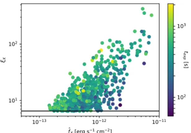
Figure 1. The measured X-ray flux fˆX and the X-ray detec- tion significanceξX, color coded by the exposure time. The black horizontal line indicates the X-ray selection criterion ξX > 6.5.

While X-ray flux and significance clearly display scaling, the scat- ter around this scaling correlates with exposure time. This rela- tion and the scatter around it can be used to estimate the X-ray selection function (c.f. section 2.3.1).

analyzed with the same source extraction tools that are em- ployed on the actual data. As a function of intrinsic flux, the fraction of recovered clusters is then used to estimate the selection functionP(X-det|f_X, ...). This process captures, to the degree that the adopted X-ray surface brightness model is consistent with that of the observed population, the im- pact of morphological variation on the selection.

In this work, we take a novel approach, inspired by the treatment of optical and SZE selection functions outlined above. This approach is based on the concept that the tradi- tional selection function can be described as a combination of two distinct statistical processes: the mapping between measured detection significance ξ_X and measured flux fˆ_X, and the mapping between measured flux fˆ_X and intrinsic flux f_X, i.e.

P(X-det|f_X, ...)=∫

dfˆ_XP(X-det|fˆ_X, ..)P(fˆ_X|f_X, ...), (17) where the second part of the integrand is the description of the measurement uncertainty of the X-ray flux. This map- ping is needed to perform the number counts and any mass calibration, so it needs to be determined anyway. Its con- struction is described in Appendix A. The first term can be easily computed from the mapping between measured flux fˆ_X and X-ray significanceξ_X,P(ξ_X|fˆ_X, ..). Indeed, it is just the cumulative distribution of that mapping forξ_X>6.5.

The mapping between measured flux fˆ_Xand X-ray sig- nificanceξ_Xcan be seen in Fig. 1 for the MARD-Y3 clusters, where we plot the detection significance against the mea- sured fluxes. The relation displays significant scatter, which is partially due to the different exposure times (color-coded).

Also clearly visible is the selection atξ_X>6.5(black line).

As an empirical model for this relation we make the ansatz hξ_Xi=ξ₀(z)e^α0 fˆ_X

f₀(z)

α1texp

400s α2

, (18)

where ξ₀(z) and f₀(z)are the median significance and mea- sured flux in redshift bins. To reduce measurement noise, we smooth them in redshift. We then assume that the signifi- cance of each cluster scatters around the mean significance

with a log-normal scatterσα. This provides the distribution P(ξ_X|fˆ_X,z,t_exp).

To fit the free parameters of this relation, namely (α₀, α₁,α₂,σ_α), we determine the likelihood of each clusterias

L_α,i = P(ξ_X⁽ⁱ⁾|fˆ_X⁽ⁱ⁾,z⁽ⁱ⁾,t_exp⁽ⁱ⁾ ) P(ξX>6.5|fˆ_X⁽ⁱ⁾,z⁽ⁱ⁾,t⁽ⁱ⁾_exp)

, (19)

where the numerator is given by evaluatingP(ξ_X|fˆ_X,z,texp) for each cluster, while the denominator ensures proper nor- malization for the actually observable data, i.e. clusters withξ_X >6.5. In properly normalising we account for the Malmquist bias introduced by the X-ray selection. Note also that we do not require the distribution of objects as a func- tion of fˆ_X to perform this fit, as it would multiply both the numerator and the denominator and hence cancel out.

The total log-likelihood of the parameters (α₀,α₁, α₂, σα) is given by the sum of the log-likelihoods lnLα = Í

ilnL_α,i. This likelihood provides stringent constraints on the parameters (α₀,α₁,α₂,σα). We find the best fitting val- uesα₀=−0.113±0.020,α₁=1.275±0.031,α₂=0.799±0.038 andσα=0.328±0.012. Noticeably, the constraints are very tight, indicating that the sample itself provides precise in- formation about this relation.

Given this relation, the X-ray selection function can be computed as

P(RASS|fˆ_X,z,t_exp)=P(ξ_X>6.5|fˆ_X,t_exp,z)

=

∫ ∞

6.5 dξ_XP(ξ_X|fˆ_X,t_exp,z). (20) Whenever the X-ray selection function is required, we sam- ple the extra nuisance parameters with the ancillary likeli- hood (Eq. 19), marginalizing over the systematic uncertain- ties in this element of the X-ray selection function. Further discussion of the parameter posteriors and their use to test for systematics in the selection function can be found in sec- tion 6.1.

2.3.2 Testing for additional dependencies

Empirically calibrating the relation governing the X-ray se- lection function has three benefits. (1) We take full account of the marginal uncertainty in the X-ray selection function.

(2) Compared to image simulation, we do not rely on the realism of the clusters put into the simulation. Indeed, we use the data themselves to infer the relation. Together with the aforementioned marginalisation this ensures that we do not artificially bias our selection function. (3) We can em- pirically explore any further trends of the residuals of the significance–flux relation with respect to other quantities.

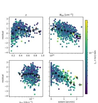
Trends of the residuals are shown in Fig. 2, where the residualσ_α⁻¹ln(ξ_X⁽ⁱ⁾/hξ_Xi⁽ⁱ⁾)is plotted against redshift (upper left panel), Galactic hydrogen column density (upper right), background count rate in an aperture of 5’ radius (lower left) and measured extent (lower right). As black dots we show the means of the populations in bins along the x axis. We find a weak trend with hydrogen column density. For simplicity we let this trend contribute to the overall scatter σ_α. We find no correlation with the background brightness. There is a clear trend with measured extent, as can be expected for extended sources like clusters. We do not, however, follow

0.2 0.4 0.6 0.8 1.0 4

3 2 1 0 1 2 3

residual

z

10²⁰

NHII [cm²]

10¹

bgr [cts s¹] 4

3 2 1 0 1 2 3

residual

0 1 2

extent [arcmin]

10¹rate [cts s]1

Figure 2.Residuals of the fitted significance–flux relation against redshift (upper left panel), Galactic foreground neutral hydrogen column density (upper right), background counts rate in the aper- ture (lower left) and measured extent. Color coded is the count rate of the objects. The residuals are normalized by the best fit value of the intrinsic scatter around the mean relation. As black point we show the means of these points in bins along the x-axis.

This plot indicates that the addition of a redshift trend or and extent trend would be natural extension of our model. The cur- rent level of systematic and statistical uncertainties however does not require these extensions.

up on this trend, as 442 of the 708 cluster that we consider have a measured extent of 0 (due to the large PSF of RASS).

Disturbingly, we find a trend with redshift which is not captured by our model, as can be seen in the upper left panel of Fig. 2. At the lowest redshifts, we tend to over predict the significance given flux and exposure time, while at intermediate and high redshifts we tend to underestimate it. This residual systematic manifests itself at different stages in our analysis, and we discuss this as it arises and again in section 6.1.

3 VALIDATION METHODS

As described above, the selection model for the clusters is specified by the form of the mass–observable relation and the intrinsic and observational scatter of the cluster popula- tion around the mean relation. The choice of the form of this relation should be driven primarily by what the data them- selves demand, with guidance from the principle of preferred simplicity (Occam’s razor) and informed by predictions from structure formation simulations. This scaling relation should be empirically calibrated using methods such as weak lensing and dynamical masses, whose systematics can be calibrated and corrected using by comparison with structure formation simulations. Finally, a key step in cosmological analyses of cluster samples is to check consistency of the cluster sample with the best fit model of cosmology and mass–observable relation (e.g., goodness of fit; see Bocquet et al. 2015).

The mass-observable relation can be calibrated using multiple sources of mass information, including direct mass information and from the cluster counts themselves (which is the distribution in observable and redshift of the clus- ter sample). thus, there is ample opportunity for validation of the scaling relation and the selection function. In future cosmology analyses, blinding of the cosmological and nuis- sance parameters will be the norm, and cluster cosmology is no exception. The validation of a cluster sample through the requirement that all different reservoirs of information about the scaling relation lead to consistent results can be carried out in a blinded manner and should lead to improved stability and robustness in the final, unblinded cosmological results. We note that given the sensitivity of mass measure- ments to the distance-redshift relation and the sensitivity of the counts to both distance-redshift and growth of structure, these blinded tests should in general be carried out within each family of cosmological models considered (e.g., flat or curvedν-ΛCDM, flat or curvedν-wCDM, etc).

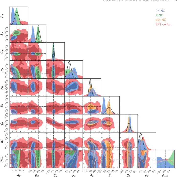
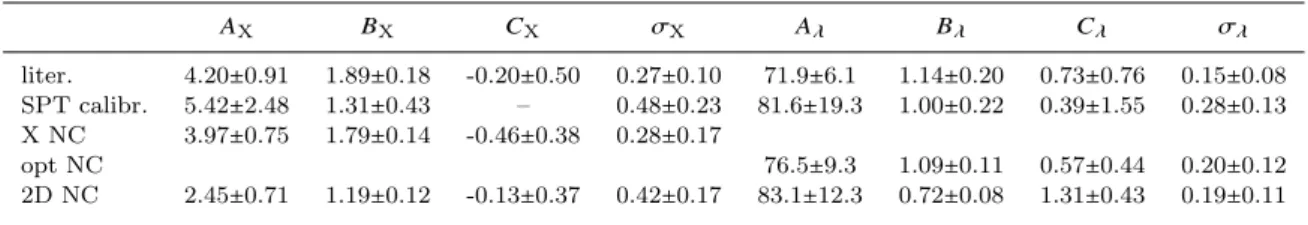
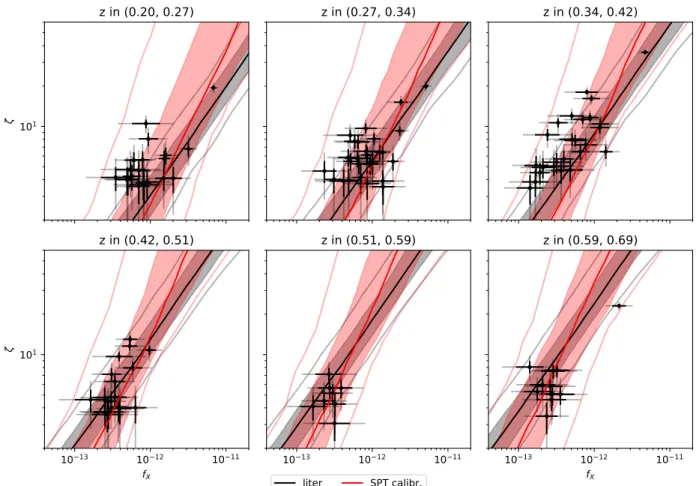
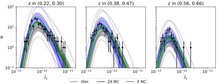
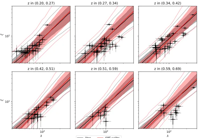
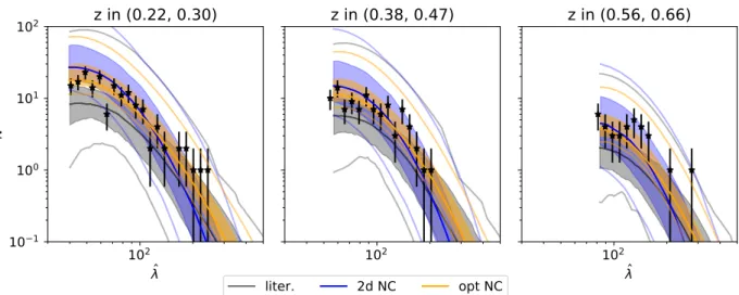
In this work we seek to perform the following tests to validate the selection function modeling of the MARD-Y3 sample: (1) we investigate whether the X-ray flux–mass and richness–mass relation obtained by cross-calibration using SPT-SZ mass information is consistent with the relation de- rived from the number counts of the MARD-Y3 sample; (2) we compare the scaling relation constraints from different flavours of number counts with each other (e.g., number counts in X-ray flux and redshift, in optical richness and red- shift, and in both X-ray flux, optical richness and redshift);

(3) finally, we constrain the probability of incompleteness in the SPT-SZ sample or contamination in the MARD-Y3 sample by comparing the clusters with and without coun- terparts in the other survey to the probabilities of having or not having counterparts as estimated using the selection functions. We take advantage in these validation tests of the fact that these scaling relations have been previously stud- ied, and so we can compare our results not only internally but also externally to the literature. Finally, a key validation test could be carried out with the weak lensing information from DES, but we delay that to a future analysis where we hope also to present unblinded cosmological results.

Given the stochastic description of the cluster popula- tion outlined above, we set-up different likelihood functions for each of these tests. These likelihoods are functions of the parameters determining the mapping between intrinsic ob- servables and mass, the scatter around these relations and the correlation coefficients among the different components of scatter. Consequently, sampling these likelihoods with the data constrains the parameters. In the following sections we present the likelihoods used for each of the three validation methods listed above.

3.1 SPT-SZ cross-calibration

For each object in the matched MARD-Y3 – SPT-SZ sam- ple (see section 4.1.3), we seek to predict the likelihood of observing the measured SZE signal-to-noise ξ⁽ⁱ⁾ given the measured X-ray flux fˆ_X⁽ⁱ⁾, measured richness λˆ⁽ⁱ⁾ and the scaling relation parameters. This likelihood is constructed by first making a prediction of the intrinsic SZE-signal-to- noiseζthat is consistent with the measured X-ray flux fˆ_X⁽ⁱ⁾

and measured richnessλˆ⁽ⁱ⁾, depending on the scaling relation parameters. To this end, the joint distribution of intrinsic properties is evaluated at the intrinsic fluxes and richnesses consistent with the measurements

P(ζ|fˆ_X⁽ⁱ⁾,λˆ⁽ⁱ⁾,z⁽ⁱ⁾) ∝

∫

dλP(λˆ⁽ⁱ⁾|λ)∫

df_XP(fˆ_X⁽ⁱ⁾|f_X) d³N

df_Xdλdζ _f

X,λ,ζ,z⁽ⁱ⁾.

(21)

This expression of expected intrinsic SZE-signal takes ac- count of the Eddington bias induced by the observational and intrinsic scatter in the X-ray and optical observable acting in combination with the fractionally larger number of objects at low mass, encoded in the last term of the ex- pression.

To evaluate the likelihood of the measured SZE signal- to-noiseξ⁽ⁱ⁾given the measured X-ray flux fˆ_X⁽ⁱ⁾and measured richnessλˆ⁽ⁱ⁾, we need to compare the predicted distribution P(ζ|fˆ_X⁽ⁱ⁾,λˆ⁽ⁱ⁾,z⁽ⁱ⁾)with the likely values of intrinsic SZE-signal derived from the measurement ξ⁽ⁱ⁾ and the measurement uncertainty. This is written

P(ξ⁽ⁱ⁾|fˆ_X⁽ⁱ⁾,λˆ⁽ⁱ⁾, z⁽ⁱ⁾)=

∫dζP(ξ⁽ⁱ⁾|ζ, γ_f⁽ⁱ⁾)P(ζ|fˆ⁽ⁱ⁾

X,λˆ⁽ⁱ⁾,z⁽ⁱ⁾)

∫dζP(SPT|ζ, γ⁽ⁱ⁾

f )P(ζ|fˆ_X⁽ⁱ⁾,λˆ⁽ⁱ⁾,z⁽ⁱ⁾)

. (22)

Notably, the denominator ensures the proper normalisation and also takes into account the Malmquist bias⁸introduced by the SPT-SZ selection. Also note that the normalization cancels the dependence of this likelihood on the amplitude of the number of objects at the redshift z⁽ⁱ⁾, measured flux

fˆ⁽ⁱ⁾

X and measured richness λˆ⁽ⁱ⁾. This strongly weakens its cosmological dependence and makes it independent of the X-ray and the optical selection function (see also Liu et al.

2015). For sake of brevity we omitted that this likelihood depends on the scaling relation parameters and the cosmo- logical parameters, all needed to compute the distribution of intrinsic properties.

The total log-likelihood of SPT-SZ cross-calibration over the matched sample is given by the sum of the indi- vidual log likelihoods

lnL_SPTcc= Õ

i∈matched

lnP(ξ⁽ⁱ⁾|fˆ_X⁽ⁱ⁾,λˆ⁽ⁱ⁾,z⁽ⁱ⁾), (23) which is a function of the scaling relation parameters and cosmology. Sampling it with priors on the SZE scaling rela- tion parameters that come from an external calibration will then transfer that calibration to the X-ray flux and richness scaling relations.

8 In cluster population studies redshift information is usually available. Thus, the term ”Malmquist bias” does not refer to the larger survey volume at which high flux objects can be detected, when compared to low flux objects. It refers to that fact that in the presence of scatter among observables, up-scattering objects are more likely to pass any selection criterion than down-scattered objects. This biases observableˆa ˘AˇTobservable plots close to the selection threshold.

3.2 Calibration with number counts

The number of clusters as a function of measured observable and redshift is a powerful way to constrain the mapping be- tween observable and mass, because the number of clusters as a function of mass is known for a given cosmology (see self-calibration discussions in Majumdar & Mohr 2003; Hu 2003; Majumdar & Mohr 2004).

3.2.1 X-ray number counts

The likelihood of number counts is given by lnL_{nc X}=Õ

i

lnN _ˆ

f_X⁽ⁱ⁾,z⁽ⁱ⁾−Ntot, (24)

where the expected number of objects as a function of mea- sured flux fˆ_X⁽ⁱ⁾and redshiftz⁽ⁱ⁾is

N _ˆ

f_X⁽ⁱ⁾,z⁽ⁱ⁾=P(RASS|fˆ_X⁽ⁱ⁾,z⁽ⁱ⁾,t⁽ⁱ⁾_exp)

∫

df_XP(fˆ_X⁽ⁱ⁾|f_X)

∫

dλP(DES|λ,z⁽ⁱ⁾) d²N df_Xdλ

fX,λ,z⁽ⁱ⁾dfˆ_X,

(25)

where the first factor takes into account the X-ray selection, the second factor models the measurement uncertainty on the X-ray flux and the third factor models the optical in- completeness.

The total number of objects is computed as Ntot=∫

dtexpP(t_exp)

∫ dz

∫

dfˆ_XP(RASS|fˆ_X,z,texp)

∫

df_XP(fˆ_X|f_X,z,texp)

∫

dλP(DES|λ,z) d²N

df_Xdλ fX,λ,z,

(26)

whereP(t_exp)is the solid angle weighted exposure time dis- tribution. We highlight here that, unlike previous work, we explicitly model not only the selection on the X-ray observ- able, but also fold in the incompleteness correction due to the MCMF optical cleaning via the termP(DES|λ,z).

3.2.2 Optical number counts

While not customary for a predominantly X-ray selected sample, the number counts of clusters can also be repre- sented as a function of optical richness.. In this case, the likelihood reads

lnL_ncλ=Õ

i

lnN

_λˆ(i),z⁽ⁱ⁾−N_tot, (27) whereN_totis given by equation( 26), whereas the expected number of clusters as a function of measured richness λˆ⁽ⁱ⁾ and redshiftz⁽ⁱ⁾is computed as follows

N _λˆ(i),z⁽ⁱ⁾=

∫

dt_expP(t_exp)

∫

dfˆ_XP(RASS|fˆ_X,z,t_exp)

∫

df_XP(fˆ_X|f_X,z,texp)

∫

dλP(λˆ⁽ⁱ⁾|λ,z) d²N df_Xdλ

fX,λ,zdλ,ˆ

(28)

where the first three integrals take account of the X-ray se- lection, while the last integral models the measurement un- certainty on the richness.

3.2.3 Combined X-ray and optical number counts

Besides determining the number counts in only one observ- able, one can also determine the number counts in more than one observable (e.g. Mantz et al. 2010), in our case by fitting for the number of objects as a function of both measured flux

fˆ⁽ⁱ⁾

X and richnessλˆ⁽ⁱ⁾. We call this flavour of number counts 2D number counts, as opposed to the 1D number counts in either X-ray flux (c.f. section 5.2.1) or richness (c.f. sec- tion 3.2.2). The likelihood of 2D number counts reads lnL_{nc X,λ}=Õ

i

lnN _ˆ

f_X⁽ⁱ⁾,λˆ⁽ⁱ⁾,z⁽ⁱ⁾−Ntot, (29)

where the expected number of objects as a function of mea- sured flux fˆ_X⁽ⁱ⁾and richnessλˆ⁽ⁱ⁾is

N _ˆ

f_X⁽ⁱ⁾,λˆ⁽ⁱ⁾,z⁽ⁱ⁾=P(RASS|fˆ_X⁽ⁱ⁾,z⁽ⁱ⁾,t_exp⁽ⁱ⁾ )

∫

df_XP(fˆ_X⁽ⁱ⁾|f_X)

∫

dλP(λˆ⁽ⁱ⁾|λ) d²N df_Xdλ

fX,λ,z⁽ⁱ⁾dfˆ_Xdλ,ˆ

(30)

computed by folding the intrinsic number density with the measurement uncertainties on flux and richness.

3.3 Consistency check using two cluster samples Given the selection functions for two cluster samples, the probability that any member of one sample is present in the other can be calculated. Thus, two distinct tests can be set up: 1) for each object in the sample A, we can compute the probability of being detected by the sample B, and com- pare this probability to the actual occurrence of matches;

2) inversely, we can start from the sample B, compute the probabilities of detection by A, and compare that to the oc- currence of matches. This provides a powerful consistency check of the two selections functions, and if anomalies are found, this approach can be used, for example, to probe for contamination or unexplained incompleteness in the cluster samples.

3.3.1 MARD-Y3 detection probability for SPT-SZ clusters For any SPT-SZ cluster with measured SZE signal-to-noise ξ⁽ⁱ⁾and redshiftz⁽ⁱ⁾in the joint SPT–DES-Y3 footprint we can compute the probability of being detected by MARD- Y3 as follows. We first predict the probability distribution of intrinsic fluxes and richnesses associated with the measured SZE-signal-to-noise as

P(f_X, λ|ξ⁽ⁱ⁾,z⁽ⁱ⁾) ∝

∫

dζP(ξ⁽ⁱ⁾|ζ, γ_f⁽ⁱ⁾) d³N df_Xdλdζ

fX,λ,ζ,z⁽ⁱ⁾.

(31)

This expression needs to be properly normalised to be a distribution in intrinsic flux and richness. This is achieved by imposing ∫

df_X∫

dλP(f_X, λ|ξ⁽ⁱ⁾,z⁽ⁱ⁾)=1, which sets the proportionality constant of the equation above. Note that this normalization cancels the dependence of this expression on the number of clusters observed.

SPT-SZ cluster ξ⁽ⁱ⁾, z⁽ⁱ⁾

should not be in MARD-Y3

should be in MARD-Y3

is not in MARD-Y3

is in MARD-Y3 1−p⁽ⁱ⁾_M|S p⁽ⁱ⁾_M|S

1−πt πt 1

(1−p⁽ⁱ⁾

M|S)(1−πt) (1−p⁽ⁱ⁾

M|S)πt+p⁽ⁱ⁾

M|S Figure 3.Probability tree describing the probability of an SPT- SZ cluster being detected in MARD-Y3. Besides the matching probability computed from the scaling between intrinsic observ- ables and mass, the scatter around this relation, the observa- tional uncertainties on the observables and the selection functions p_M|S⁽ⁱ⁾ , we also introduce the chance of either X-ray flux and rich- ness boosting or SZE signal dimmingπt, which would lead to the MARD-Y3 detection of SPT-SZ cluster that should otherwise not have been matched. Summarized at the end of each branch are the probabilities of matching or of not matching.

The predicted distribution of intrinsic fluxes and rich- nesses needs to be folded with the selection functions to com- pute the detection probability. The optical selection function is simply given by equation (15) evaluated at the cluster redshiftz⁽ⁱ⁾. On the other hand, when computing the X-ray selection function we take the RASS exposure time at the SPT-SZ position into account, while marginalising over all possible measured fluxes. The X-ray selection function thus reads

P(RASS|f_X,t_exp⁽ⁱ⁾ ,z⁽ⁱ⁾)=

∫

dfˆ_XP(RASS|fˆ_X,t⁽ⁱ⁾_exp,z⁽ⁱ⁾) P(fˆ_X|f_X,t⁽ⁱ⁾_exp,z⁽ⁱ⁾),

(32)

where the second factor is taken from equation (11), the ex- pression for the X-ray measurement error at arbitrary mea- sured flux fˆ_X.

The probability of detecting in MARD-Y3 a SPT-SZ cluster with measured SZE-signal-to-noiseξ⁽ⁱ⁾ and redshift z⁽ⁱ⁾can then be computed by folding the predicted distribu- tion of fluxes and richnesses with the selection functions in flux and richness as follows

p⁽ⁱ⁾_M|S:=P(RASS,DES|ξ⁽ⁱ⁾,z⁽ⁱ⁾)

=∫

df_XP(RASS|f_X,t⁽ⁱ⁾_exp,z⁽ⁱ⁾)

∫

dλP(DES|λ,z⁽ⁱ⁾)P(f_X, λ|ξ⁽ⁱ⁾,z⁽ⁱ⁾),

(33)

where we omit the dependence on the SPT-SZ field depth γ⁽ⁱ⁾_f at the position of the SPT-SZ selected cluster.

Given these probabilities, we can define two interesting classes of objects: (1)unexpected MARD-Y3 confirmations of SPT-SZ detections, i.e. SPT-SZ objects that should not have a MARD-Y3 match given their low probability but

MARD-Y3 objectfˆ_X⁽ⁱ⁾, λˆ⁽ⁱ⁾,z⁽ⁱ⁾

is contaminant is cluster

should not be in SPT-SZ

should be in SPT-SZ

is not in

SPT-SZ is in SPT-SZ

πc 1−πc

1−p_S|M⁽ⁱ⁾ p_S|M⁽ⁱ⁾

1 πi 1−πi

1

πc+(1−πc)(1−p_S|M⁽ⁱ⁾ +πip_S|M⁽ⁱ⁾ ) (1−πc)p⁽ⁱ⁾_S|M(1−πi) Figure 4.Probability tree describing the probability of a MARD- Y3 cluster being detected by SPT. Besides the matching probabil- ity computed from the scaling between intrinsic observables and mass, the scatter around this relation, the observational uncer- tainties on the observables and the selection functions p_S|M⁽ⁱ⁾ , we also introduce the chance that a MARD-Y3 cluster is a contam- inant πc, and the chance that SPT-SZ misses a cluster that it should detect, indicating incompleteness in SPT,πi. Summarized at the end of each branch are the probabilities of being matched or not matched.

have been nonetheless matched , and (2)missed MARD-Y3 confirmations of SPT-SZ detections, i.e SPT-SZ objects with a very high chance of being matched by MARD-Y3 that have nonetheless not been matched. For the discussion in this pa- per we adopt a low probability threshold ofp⁽_M|Sⁱ⁾ <0.025for the unexpected confirmations, and we adopt a high probabil- ity threshold ofp⁽_M|Sⁱ⁾ >0.975for the missed confirmations.

Anticipating that we find a few unexpected MARD- Y3 confirmations and no missed confirmations, we introduce here the probabilityπt that an SPT-SZ cluster that should not be confirmed based on his p⁽ⁱ⁾_M|S is confirmed nonethe- less. The likelihood ofπtcan be computed by following the probability tree shown in Fig 3. The probability of being matched is(1−p⁽ⁱ⁾_M|S)πt+p⁽ⁱ⁾_M|S, while the probability of not being matched is(1−p⁽_M|Sⁱ⁾ )(1−πt). Thus, the log-likelihood is given by

lnL(π_t)= Õ

i∈match

ln (1−p⁽_M|Sⁱ⁾ )π_t+p⁽_M|Sⁱ⁾ +

+ Õ

i∈!match

ln (1−p⁽_M|Sⁱ⁾ )(1−πt)

(34)

This likelihood also depends on the scaling relation parame- ters through the detection probabilitiesp⁽_M|Sⁱ⁾ . Marginalizing over these scaling relation parameters accounts for the sys- tematic uncertainty on the observable–mass relations.

3.3.2 SPT-SZ detection probability for MARD-Y3 clusters Similarly to the case in the previous section, for each MARD- Y3 cluster with measured X-ray flux fˆ_X⁽ⁱ⁾, measured richness

λˆ⁽ⁱ⁾and redshiftz⁽ⁱ⁾in the joint SPT-SZ–DES-Y3 footprint, we can compute the probability of it being detected by SPT

p⁽_S|Mⁱ⁾ :=P(SPT|fˆ_X⁽ⁱ⁾,λˆ⁽ⁱ⁾,z⁽ⁱ⁾)

=

∫

dζP(SPT|ζ, γ_f⁽ⁱ⁾)P(ζ|fˆ_X⁽ⁱ⁾,λˆ⁽ⁱ⁾,z⁽ⁱ⁾), (35) where the first factor in the integrand is the SPT-SZ selec- tion function evaluated for the field depth at the MARD-Y3 cluster position, while the second factor is the prediction for the intrinsic SZE-signal-to-noise consistent with the mea- sured X-ray and optical properties. The latter is taken from equation (21) while ensuring that it is properly normalized,

∫dζP(ζ|fˆ⁽ⁱ⁾

X,λˆ⁽ⁱ⁾)=1.

We introduce the probability of each individual MARD- Y3 cluster being a contaminantπc, and the probability that a SPT-SZ cluster that should be detected has not been de- tected π_i. From the probability tree shown in Fig. 4 we can determine the probability of a MARD-Y3 cluster being matched by SPT-SZ as(1−πc)p⁽ⁱ⁾

S|M(1−π_i), and the prob- ability of a cluster not being matched as πc+(1−πc)(1− p⁽ⁱ⁾_S|M+π_ip⁽ⁱ⁾_S|M). Thus, the log-likelihood is given by

lnL(πc, π_i)= Õ

i∈match

ln

(1−πc)p⁽ⁱ⁾

S|M(1−π_i) + Õ

i∈!match

ln(πc+(1−πc)(1−p⁽ⁱ⁾_S|M+πip⁽ⁱ⁾_S|M)).

(36) This likelihood also depends on the scaling relation parame- ter through the detection probabilitiesp⁽ⁱ⁾_M|S. Marginalizing over the scaling relation parameters accounts for the the systematic uncertainties on the observable–mass relations.

Finally, note that the probability of MARD-Y3 contamina- tionπc and of SPT incompletenessπ_iare perfectly degen- erate in this context. We find that the likelihood of SPT confirmation of MARD-Y3 clusters (Eq. 36) effectively only constrains the difference between the two probabilities. That isπc=0.1andπ_i=0.0is approximately as likely asπc=0.0 andπ_i=0.1.

3.3.3 Physical Interpretation

Several physical effects might bias cluster observables in an unusually significant level compared to the exception from the scatter in observables. In the case of the X-ray flux these effects are, for instance, AGN contamination and clus- ter core phenomena. Line of sight projections might bias the richness of an object, while extreme astrophysical con- tamination from correlated radio or dusty emission might bias the SZE signal. The object classes defined above (sec- tion 3.3.1 and 3.3.2) allow one to select likely candidates for these effects from the comparison of two surveys. This is especially useful in the low signal-to-noise regime where the mass incompleteness of cluster samples in large. In this regime, physical effects within clusters are not resolved. Se- lecting target lists for high signal-to-noise follow-up might thus further our understanding on the mass incompleteness.

For instance, the classification as an unexpected MARD-Y3 confirmations of an SPT-SZ object can be due to